
An official website of the United States government
The .gov means it’s official. Federal government websites often end in .gov or .mil. Before sharing sensitive information, make sure you’re on a federal government site.
The site is secure. The https:// ensures that you are connecting to the official website and that any information you provide is encrypted and transmitted securely.
- Publications
- Account settings
Preview improvements coming to the PMC website in October 2024. Learn More or Try it out now .
- Advanced Search
- Journal List
- Int J Endocrinol Metab
- v.10(2); Spring 2012

Normality Tests for Statistical Analysis: A Guide for Non-Statisticians
Asghar ghasemi.
1 Endocrine Research Center, Research Institute for Endocrine Sciences, Shahid Beheshti University of Medical Sciences, Tehran, IR Iran
Saleh Zahediasl
Statistical errors are common in scientific literature and about 50% of the published articles have at least one error. The assumption of normality needs to be checked for many statistical procedures, namely parametric tests, because their validity depends on it. The aim of this commentary is to overview checking for normality in statistical analysis using SPSS.
1. Background
Statistical errors are common in scientific literature, and about 50% of the published articles have at least one error ( 1 ). Many of the statistical procedures including correlation, regression, t tests, and analysis of variance, namely parametric tests, are based on the assumption that the data follows a normal distribution or a Gaussian distribution (after Johann Karl Gauss, 1777–1855); that is, it is assumed that the populations from which the samples are taken are normally distributed ( 2 - 5 ). The assumption of normality is especially critical when constructing reference intervals for variables ( 6 ). Normality and other assumptions should be taken seriously, for when these assumptions do not hold, it is impossible to draw accurate and reliable conclusions about reality ( 2 , 7 ).
With large enough sample sizes (> 30 or 40), the violation of the normality assumption should not cause major problems ( 4 ); this implies that we can use parametric procedures even when the data are not normally distributed ( 8 ). If we have samples consisting of hundreds of observations, we can ignore the distribution of the data ( 3 ). According to the central limit theorem, (a) if the sample data are approximately normal then the sampling distribution too will be normal; (b) in large samples (> 30 or 40), the sampling distribution tends to be normal, regardless of the shape of the data ( 2 , 8 ); and (c) means of random samples from any distribution will themselves have normal distribution ( 3 ). Although true normality is considered to be a myth ( 8 ), we can look for normality visually by using normal plots ( 2 , 3 ) or by significance tests, that is, comparing the sample distribution to a normal one ( 2 , 3 ). It is important to ascertain whether data show a serious deviation from normality ( 8 ). The purpose of this report is to overview the procedures for checking normality in statistical analysis using SPSS.
2. Visual Methods
Visual inspection of the distribution may be used for assessing normality, although this approach is usually unreliable and does not guarantee that the distribution is normal ( 2 , 3 , 7 ). However, when data are presented visually, readers of an article can judge the distribution assumption by themselves ( 9 ). The frequency distribution (histogram), stem-and-leaf plot, boxplot, P-P plot (probability-probability plot), and Q-Q plot (quantile-quantile plot) are used for checking normality visually ( 2 ). The frequency distribution that plots the observed values against their frequency, provides both a visual judgment about whether the distribution is bell shaped and insights about gaps in the data and outliers outlying values ( 10 ). The stem-and-leaf plot is a method similar to the histogram, although it retains information about the actual data values ( 8 ). The P-P plot plots the cumulative probability of a variable against the cumulative probability of a particular distribution (e.g., normal distribution). After data are ranked and sorted, the corresponding z-score is calculated for each rank as follows: z = x - ᵪ̅ / s . This is the expected value that the score should have in a normal distribution. The scores are then themselves converted to z-scores. The actual z-scores are plotted against the expected z-scores. If the data are normally distributed, the result would be a straight diagonal line ( 2 ). A Q-Q plot is very similar to the P-P plot except that it plots the quantiles (values that split a data set into equal portions) of the data set instead of every individual score in the data. Moreover, the Q-Q plots are easier to interpret in case of large sample sizes ( 2 ). The boxplot shows the median as a horizontal line inside the box and the interquartile range (range between the 25 th to 75 th percentiles) as the length of the box. The whiskers (line extending from the top and bottom of the box) represent the minimum and maximum values when they are within 1.5 times the interquartile range from either end of the box ( 10 ). Scores greater than 1.5 times the interquartile range are out of the boxplot and are considered as outliers, and those greater than 3 times the interquartile range are extreme outliers. A boxplot that is symmetric with the median line at approximately the center of the box and with symmetric whiskers that are slightly longer than the subsections of the center box suggests that the data may have come from a normal distribution ( 8 ).
3. Normality Tests
The normality tests are supplementary to the graphical assessment of normality ( 8 ). The main tests for the assessment of normality are Kolmogorov-Smirnov (K-S) test ( 7 ), Lilliefors corrected K-S test ( 7 , 10 ), Shapiro-Wilk test ( 7 , 10 ), Anderson-Darling test ( 7 ), Cramer-von Mises test ( 7 ), D’Agostino skewness test ( 7 ), Anscombe-Glynn kurtosis test ( 7 ), D’Agostino-Pearson omnibus test ( 7 ), and the Jarque-Bera test ( 7 ). Among these, K-S is a much used test ( 11 ) and the K-S and Shapiro-Wilk tests can be conducted in the SPSS Explore procedure (Analyze → Descriptive Statistics → Explore → Plots → Normality plots with tests) ( 8 ).
The tests mentioned above compare the scores in the sample to a normally distributed set of scores with the same mean and standard deviation; the null hypothesis is that “sample distribution is normal.” If the test is significant, the distribution is non-normal. For small sample sizes, normality tests have little power to reject the null hypothesis and therefore small samples most often pass normality tests ( 7 ). For large sample sizes, significant results would be derived even in the case of a small deviation from normality ( 2 , 7 ), although this small deviation will not affect the results of a parametric test ( 7 ). The K-S test is an empirical distribution function (EDF) in which the theoretical cumulative distribution function of the test distribution is contrasted with the EDF of the data ( 7 ). A limitation of the K-S test is its high sensitivity to extreme values; the Lilliefors correction renders this test less conservative ( 10 ). It has been reported that the K-S test has low power and it should not be seriously considered for testing normality ( 11 ). Moreover, it is not recommended when parameters are estimated from the data, regardless of sample size ( 12 ).
The Shapiro-Wilk test is based on the correlation between the data and the corresponding normal scores ( 10 ) and provides better power than the K-S test even after the Lilliefors correction ( 12 ). Power is the most frequent measure of the value of a test for normality—the ability to detect whether a sample comes from a non-normal distribution ( 11 ). Some researchers recommend the Shapiro-Wilk test as the best choice for testing the normality of data ( 11 ).
4. Testing Normality Using SPSS
We consider two examples from previously published data: serum magnesium levels in 12–16 year old girls (with normal distribution, n = 30) ( 13 ) and serum thyroid stimulating hormone (TSH) levels in adult control subjects (with non-normal distribution, n = 24) ( 14 ). SPSS provides the K-S (with Lilliefors correction) and the Shapiro-Wilk normality tests and recommends these tests only for a sample size of less than 50 ( 8 ).
In Figure , both frequency distributions and P-P plots show that serum magnesium data follow a normal distribution while serum TSH levels do not. Results of K-S with Lilliefors correction and Shapiro-Wilk normality tests for serum magnesium and TSH levels are shown in Table . It is clear that for serum magnesium concentrations, both tests have a p-value greater than 0.05, which indicates normal distribution of data, while for serum TSH concentrations, data are not normally distributed as both p values are less than 0.05. Lack of symmetry (skewness) and pointiness (kurtosis) are two main ways in which a distribution can deviate from normal. The values for these parameters should be zero in a normal distribution. These values can be converted to a z-score as follows:

| No. | Mean ± SD | Mean ± SEM | Skewness | SE | Z | Kurtosis | SE | Z | K-S With Lilliefors Correction Test | Shapiro-Wilk Test | ||||||
|---|---|---|---|---|---|---|---|---|---|---|---|---|---|---|---|---|
| Statistics | Df | value | Statistics | Df | -value | |||||||||||
| Serum magnesium, mg/dL | 30 | 2.08 ± 0.175 | 2.08 ± 0.03 | 0.745 | 0.427 | 1.74 | 0.567 | 0.833 | 0.681 | 0.137 | 30 | 0.156 | 0.955 | 30 | 0.236 | |
| Serum TSH , mU/L | 24 | 1.67 ± 1.53 | 1.67 ± 0.31 | 1.594 | 0.472 | 3.38 | 1.401 | 0.918 | 1.52 | 0.230 | 24 | 0.002 | 0.750 | 24 | <0.001 | |
a Abbreviations: Df, Degree of freedom; K-S, Kolmogorov-Smirnov; SD, Standard deviation; SEM, Standard error of mean; TSH, Thyroid stimulating hormone
Z Skewness = Skewness-0 / SE Skewness and Z Kurtosis = Kurtosis-0 / SE Kurtosis .
An absolute value of the score greater than 1.96 or lesser than -1.96 is significant at P < 0.05, while greater than 2.58 or lesser than -2.58 is significant at P < 0.01, and greater than 3.29 or lesser than -3.29 is significant at P < 0.001. In small samples, values greater or lesser than 1.96 are sufficient to establish normality of the data. However, in large samples (200 or more) with small standard errors, this criterion should be changed to ± 2.58 and in very large samples no criterion should be applied (that is, significance tests of skewness and kurtosis should not be used) ( 2 ). Results presented in Table indicate that parametric statistics should be used for serum magnesium data and non-parametric statistics should be used for serum TSH data.
5. Conclusions
According to the available literature, assessing the normality assumption should be taken into account for using parametric statistical tests. It seems that the most popular test for normality, that is, the K-S test, should no longer be used owing to its low power. It is preferable that normality be assessed both visually and through normality tests, of which the Shapiro-Wilk test, provided by the SPSS software, is highly recommended. The normality assumption also needs to be considered for validation of data presented in the literature as it shows whether correct statistical tests have been used.
Acknowledgments
The authors thank Ms. N. Shiva for critical editing of the manuscript for English grammar and syntax and Dr. F. Hosseinpanah for statistical comments.
Implication for health policy/practice/research/medical education: Data presented in this article could help for the selection of appropriate statistical analyses based on the distribution of data.
Please cite this paper as: Ghasemi A, Zahediasl S. Normality Tests for Statistical Analysis: A Guide for Non-Statisticians. Int J Endocrinol Metab. 2012;10(2):486-9. DOI: 10.5812/ijem.3505
Financial Disclosure: None declared.
Funding/Support: None declared.
Normality test
One of the most common assumptions for statistical tests is that the data used are normally distributed. For example, if you want to run a t-test or an ANOVA , you must first test whether the data or variables are normally distributed.
The assumption of normal distribution is also important for linear regression analysis , but in this case it is important that the error made by the model is normally distributed, not the data itself.
Nonparametric tests
If the data are not normally distributed, the above procedures cannot be used and non-parametric tests must be used. Non-parametric tests do not assume that the data are normally distributed.
How is the normal distribution tested?
Normal distribution can be tested either analytically (statistical tests) or graphically. The most common analytical tests to check data for normal distribution are the:
- Kolmogorov-Smirnov Test
- Shapiro-Wilk Test
- Anderson-Darling Test
For graphical verification, either a histogram or, better, the Q-Q plot is used. Q-Q stands for quantile-quantile plot, where the actually observed distribution is compared with the theoretically expected distribution.
Statistical tests for normal distribution
To test your data analytically for normal distribution, there are several test procedures, the best known being the Kolmogorov-Smirnov test, the Shapiro-Wilk test, and the Anderson Darling test.

In all of these tests, you are testing the null hypothesis that your data are normally distributed. The null hypothesis is that the frequency distribution of your data is normally distributed. To reject or not reject the null hypothesis, all these tests give you a p-value . What matters is whether this p-value is less than or greater than 0.05.

If the p-value is less than 0.05, this is interpreted as a significant deviation from the normal distribution and it can be assumed that the data are not normally distributed. If the p-value is greater than 0.05 and you want to be statistically clean, you cannot necessarily say that the frequency distribution is normal, you just cannot reject the null hypothesis.
In practice, a normal distribution is assumed for values greater than 0.05, although this is not entirely correct. Nevertheless, the graphical solution should always be considered.
Note: The Kolmogorov-Smirnov test and the Anderson-Darling test can also be used to test distributions other than the normal distribution.
Disadvantage of the analytical tests for normal distribution
Unfortunately, the analytical method has a major drawback, which is why more and more attention is being paid to graphical methods.
The problem is that the calculated p-value is affected by the size of the sample. Therefore, if you have a very small sample, your p-value may be much larger than 0.05, but if you have a very very large sample from the same population, your p-value may be smaller than 0.05.

If we assume that the distribution in the population deviates only slightly from the normal distribution, we will get a very large p-value with a very small sample and therefore assume that the data are normally distributed. However, if you take a larger sample, the p-value gets smaller and smaller, even though the samples are from the same population with the same distribution. With a very large sample, you can even get a p-value of less than 0.05, rejecting the null hypothesis of normal distribution.
To avoid this problem, graphical methods are increasingly being used.
Graphical test for normal distribution
If the normal distribution is tested graphically, one looks either at the histogram or even better the QQ plot.
If you want to check the normal distribution using a histogram, plot the normal distribution on the histogram of your data and check that the distribution curve of the data approximately matches the normal distribution curve.

A better way to do this is to use a quantile-quantile plot, or Q-Q plot for short. This compares the theoretical quantiles that the data should have if they were perfectly normal with the quantiles of the measured values.

If the data were perfectly normally distributed, all points would lie on the line. The further the data deviates from the line, the less normally distributed the data is.
In addition, DATAtab plots the 95% confidence interval. If all or almost all of the data fall within this interval, this is a very strong indication that the data are normally distributed. They are not normally distributed if, for example, they form an arc and are far from the line in some areas.
Test Normal distribution in DATAtab
When you test your data for normal distribution with DATAtab, you get the following evaluation, first the analytical test procedures clearly arranged in a table, then the graphical test procedures.

If you want to test your data for normal distribution, simply copy your data into the table on DATAtab, click on descriptive statistics and then select the variable you want to test for normal distribution. Then, just click on Test Normal Distribution and you will get the results.
Furthermore, if you are calculating a hypothesis test with DATAtab, you can test the assumptions for each hypothesis test, if one of the assumptions is the normal distribution, then you will get the test for normal distribution in the same way.
Statistics made easy
- many illustrative examples
- ideal for exams and theses
- statistics made easy on 412 pages
- 5rd revised edition (April 2024)
- Only 7.99 €

"Super simple written"
"It could not be simpler"
"So many helpful examples"

Cite DATAtab: DATAtab Team (2024). DATAtab: Online Statistics Calculator. DATAtab e.U. Graz, Austria. URL https://datatab.net
Best Practice: How to Write a Dissertation or Thesis Quantitative Chapter 4
Statistics Blog
In the first paragraph of your quantitative chapter 4, the results chapter, restate the research questions that will be examined. This reminds the reader of what you’re going to investigate after having been trough the details of your methodology. It’s helpful too that the reader knows what the variables are that are going to be analyzed.
Spend a paragraph telling the reader how you’re going to clean the data. Did you remove univariate or multivariate outlier? How are you going to treat missing data? What is your final sample size?
The next paragraph should describe the sample using demographics and research variables. Provide frequencies and percentages for nominal and ordinal level variables and means and standard deviations for the scale level variables. You can provide this information in figures and tables.
Here’s a sample:
Frequencies and Percentages. The most frequently observed category of Cardio was Yes ( n = 41, 72%). The most frequently observed category of Shock was No ( n = 34, 60%). Frequencies and percentages are presented.
Summary Statistics. The observations for MiniCog had an average of 25.49 ( SD = 14.01, SE M = 1.87, Min = 2.00, Max = 55.00). The observations for Digital had an average of 29.12 ( SD = 10.03, SE M = 1.33, Min = 15.50, Max = 48.50). Skewness and kurtosis were also calculated. When the skewness is greater than 2 in absolute value, the variable is considered to be asymmetrical about its mean. When the kurtosis is greater than or equal to 3, then the variable’s distribution is markedly different than a normal distribution in its tendency to produce outliers (Westfall & Henning, 2013).
Now that the data is clean and descriptives have been conducted, turn to conducting the statistics and assumptions of those statistics for research question 1. Provide the assumptions first, then the results of the statistics. Have a clear accept or reject of the hypothesis statement if you have one. Here’s an independent samples t-test example:
Introduction. An two-tailed independent samples t -test was conducted to examine whether the mean of MiniCog was significantly different between the No and Yes categories of Cardio.
Assumptions. The assumptions of normality and homogeneity of variance were assessed.
Normality. A Shapiro-Wilk test was conducted to determine whether MiniCog could have been produced by a normal distribution (Razali & Wah, 2011). The results of the Shapiro-Wilk test were significant, W = 0.94, p = .007. These results suggest that MiniCog is unlikely to have been produced by a normal distribution; thus normality cannot be assumed. However, the mean of any random variable will be approximately normally distributed as sample size increases according to the Central Limit Theorem (CLT). Therefore, with a sufficiently large sample size ( n > 50), deviations from normality will have little effect on the results (Stevens, 2009). An alternative way to test the assumption of normality was utilized by plotting the quantiles of the model residuals against the quantiles of a Chi-square distribution, also called a Q-Q scatterplot (DeCarlo, 1997). For the assumption of normality to be met, the quantiles of the residuals must not strongly deviate from the theoretical quantiles. Strong deviations could indicate that the parameter estimates are unreliable. Figure 1 presents a Q-Q scatterplot of MiniCog.
Homogeneity of variance. Levene’s test for equality of variance was used to assess whether the homogeneity of variance assumption was met (Levene, 1960). The homogeneity of variance assumption requires the variance of the dependent variable be approximately equal in each group. The result of Levene’s test was significant, F (1, 54) = 18.30, p < .001, indicating that the assumption of homogeneity of variance was violated. Consequently, the results may not be reliable or generalizable. Since equal variances cannot be assumed, Welch’s t-test was used instead of the Student’s t-test, which is more reliable when the two samples have unequal variances and unequal sample sizes (Ruxton, 2006).
Results. The result of the two-tailed independent samples t -test was significant, t (46.88) = -4.81, p < .001, indicating the null hypothesis can be rejected. This finding suggests the mean of MiniCog was significantly different between the No and Yes categories of Cardio. The mean of MiniCog in the No category of Cardio was significantly lower than the mean of MiniCog in the Yes category. Present the results of the two-tailed independent samples t -test, and present the means of MiniCog(No) and MiniCog(Yes).
In the next paragraphs, conduct stats and assumptions for your other research questions. Again, assumptions first, then the results of the statistics with appropriate tables and figures.
Be sure to add all of the in-text citations to your reference section. Here is a sample of references.
Conover, W. J., & Iman, R. L. (1981). Rank transformations as a bridge between parametric and nonparametric statistics. The American Statistician, 35 (3), 124-129.
DeCarlo, L. T. (1997). On the meaning and use of kurtosis. Psychological Methods, 2(3), 292-307.
Levene, H. (1960). Contributions to Probability and Statistics. Essays in honor of Harold Hotelling, I. Olkin et al. eds., Stanford University Press, 278-292.
Razali, N. M., & Wah, Y. B. (2011). Power comparisons of Shapiro-Wilk, Kolmogorov-Smirnov, Lilliefors and Anderson-Darling tests. Journal of Statistical Modeling and Analytics, 2 (1), 21-33.
Ruxton, G. D. (2006). The unequal variance t-test is an underused alternative to Student’s t-test and the Mann-Whitney U test. Behavioral Ecology, 17 (4), 688-690.
Intellectus Statistics [Online computer software]. (2019). Retrieved from https://analyze.intellectusstatistics.com/
Stevens, J. P. (2009). Applied multivariate statistics for the social sciences (5th ed.). Mahwah, NJ: Routledge Academic.
Westfall, P. H., & Henning, K. S. S. (2013). Texts in statistical science: Understanding advanced statistical methods. Boca Raton, FL: Taylor & Francis.
Teach yourself statistics
How to Test for Normality: Three Simple Tests
Many statistical techniques (regression, ANOVA, t-tests, etc.) rely on the assumption that data is normally distributed. For these techniques, it is good practice to examine the data to confirm that the assumption of normality is tenable.
With that in mind, here are three simple ways to test interval-scale data or ratio-scale data for normality.
- Check descriptive statistics.
- Generate a histogram.
- Conduct a chi-square test.
Each option is easy to implement with Excel, as long as you have Excel's Analysis ToolPak.
The Analysis ToolPak
To conduct the tests for normality described below, you need a free Microsoft add-in called the Analysis ToolPak, which may or may not be already installed on your copy of Excel.
To determine whether you have the Analysis ToolPak, click the Data tab in the main Excel menu. If you see Data Analysis in the Analysis section, you're good. You have the ToolPak.
If you don't have the ToolPak, you need to get it. Go to: How to Install the Data Analysis ToolPak in Excel .
Descriptive Statistics
Perhaps, the easiest way to test for normality is to examine several common descriptive statistics. Here's what to look for:
- Central tendency. The mean and the median are summary measures used to describe central tendency - the most "typical" value in a set of values. With a normal distribution, the mean is equal to the median.
- Skewness. Skewness is a measure of the asymmetry of a probability distribution. If observations are equally distributed around the mean, the skewness value is zero; otherwise, the skewness value is positive or negative. As a rule of thumb, skewness between -2 and +2 is consistent with a normal distribution.
- Kurtosis. Kurtosis is a measure of whether observations cluster around the mean of the distribution or in the tails of the distribution. The normal distribution has a kurtosis value of zero. As a rule of thumb, kurtosis between -2 and +2 is consistent with a normal distribution.
Together, these descriptive measures provide a useful basis for judging whether a data set satisfies the assumption of normality.
To see how to compute descriptive statistics in Excel, consider the following data set:
| Sample data | ||||
|---|---|---|---|---|
| 1 2 3 3 3.5 | 4 4 5 5 5 | 5.5 5.5 6 6 6 | 6.5 7 7 8 9 | |
Begin by entering data in a column or row of an Excel spreadsheet:
Next, from the navigation menu in Excel, click Data / Data analysis . That displays the Data Analysis dialog box. From the Data Analysis dialog box, select Descriptive Statistics and click the OK button:
Then, in the Descriptive Statistics dialog box, enter the input range, and click the Summary Statistics check box. The dialog box, with entries, should look like this:
And finally, to display summary statistics, click the OK button on the Descriptive Statistics dialog box. Among other outputs, you should see the following:
The mean is nearly equal to the median. And both skewness and kurtosis are between -2 and +2.
Conclusion: These descriptive statistics are consistent with a normal distribution.
Another easy way to test for normality is to plot data in a histogram , and see if the histogram reveals the bell-shaped pattern characteristic of a normal distribution. With Excel, this is a a four-step process:
- Enter data. This means entering data values in an Excel spreadsheet. The column, row, or range of cells that holds data is the input range .
- Define bins. In Excel, bins are category ranges. To define a bin, you enter the upper range of each bin in a column, row, or range of cells. The block of cells that holds upper-range entries is called the bin range .
- Plot the data in a histogram. In Excel, access the histogram function through: Data / Data analysis / Histogram .
- In the Histogram dialog box, enter the input range and the bin range ; and check the Chart Output box. Then, click OK.
If the resulting histogram looks like a bell-shaped curve, your work is done. The data set is normal or nearly normal. If the curve is not bell-shaped, the data may not be normal.
To see how to plot data for normality with a histogram in Excel, we'll use the same data set (shown below) that we used in Example 1.
Begin by entering data to define an input range and a bin range. Here is what data entry looks like in an Excel spreadsheet:
Next, from the navigation menu in Excel, click Data / Data analysis . That displays the Data Analysis dialog box. From the Data Analysis dialog box, select Histogram and click the OK button:
Then, in the Histogram dialog box, enter the input range, enter the bin range, and click the Chart Output check box. The dialog box, with entries, should look like this:
And finally, to display the histogram, click the OK button on the Histogram dialog box. Here is what you should see:
The plot is fairly bell-shaped - an almost-symmetric pattern with one peak in the middle. Given this result, it would be safe to assume that the data were drawn from a normal distribution. On the other hand, if the plot were not bell-shaped, you might suspect the data were not from a normal distribution.
Chi-Square Test
The chi-square test for normality is another good option for determining whether a set of data was sampled from a normal distribution.
Note: All chi-square tests assume that the data under investigation was sampled randomly.
Hypothesis Testing
The chi-square test for normality is an actual hypothesis test , where we examine observed data to choose between two statistical hypotheses:
- Null hypothesis: Data is sampled from a normal distribution.
- Alternative hypothesis: Data is not sampled from a normal distribution.
Like many other techniques for testing hypotheses, the chi-square test for normality involves computing a test-statistic and finding the P-value for the test statistic, given degrees of freedom and significance level . If the P-value is bigger than the significance level, we accept the null hypothesis; if it is smaller, we reject the null hypothesis.
How to Conduct the Chi-Square Test
The steps required to conduct a chi-square test of normality are listed below:
- Specify the significance level.
- Find the mean, standard deviation, sample size for the sample.
- Define non-overlapping bins.
- Count observations in each bin, based on actual dependent variable scores.
- Find the cumulative probability for each bin endpoint.
- Find the probability that an observation would land in each bin, assuming a normal distribution.
- Find the expected number of observations in each bin, assuming a normal distribution.
- Compute a chi-square statistic.
- Find the degrees of freedom, based on the number of bins.
- Find the P-value for the chi-square statistic, based on degrees of freedom.
- Accept or reject the null hypothesis, based on P-value and significance level.
So you will understand how to accomplish each step, let's work through an example, one step at a time.
To demonstrate how to conduct a chi-square test for normality in Excel, we'll use the same data set (shown below) that we've used for the previous two examples. Here it is again:
Now, using this data, let's check for normality.
Specify Significance Level
The significance level is the probability of rejecting the null hypothesis when it is true. Researchers often choose 0.05 or 0.01 for a significance level. For the purpose of this exercise, let's choose 0.05.
Find the Mean, Standard Deviation, and Sample Size
To compute a chi-square test statistic, we need to know the mean, standared deviation, and sample size. Excel can provide this information. Here's how:
Define Bins
To conduct a chi-square analysis, we need to define bins, based on dependent variable scores. Each bin is defined by a non-overlapping range of values.
For the chi-square test to be valid, each bin should hold at least five observations. With that in mind, we'll define four bins for this example, as shown below:
Bin 1 will hold dependent variable scores that are less than 4; Bin 2, scores between 4 and 5; Bin 3, scores between 5.1 and 6; and and Bin 4, scores greater than 6.
Note: The number of bins is an arbitrary decision made by the experimenter, as long as the experimenter chooses at least four bins and at least five observations per bin. With fewer than four bins, there are not enough degrees of freedom for the analysis. For this example, we chose to define only four bins. Given the small sample, if we used more bins, at least one bin would have fewer than five observations per bin.
Count Observed Data Points in Each Bin
The next step is to count the observed data points in each bin. The figure below shows sample observations allocated to bins, with a frequency count for each bin in the final row.
Note: We have five observed data points in each bin - the minimum required for a valid chi-square test of normality.
Find Cumulative Probability
A cumulative probability refers to the probability that a random variable is less than or equal to a specific value. In Excel, the NORMDIST function computes cumulative probabilities from a normal distribution.
Assuming our data follows a normal distribution, we can use the NORMDIST function to find cumulative probabilities for the upper endpoints in each bin. Here is the formula we use:
P j = NORMDIST (MAX j , X , s, TRUE)
where P j is the cumulative probability for the upper endpoint in Bin j , MAX j is the upper endpoint for Bin j , X is the mean of the data set, and s is the standard deviation of the data set.
When we execute the formula in Excel, we get the following results:
P 1 = NORMDIST (4, 5.1, 2.0, TRUE) = 0.29
P 2 = NORMDIST (5, 5.1, 2.0, TRUE) = 0.48
P 3 = NORMDIST (6, 5.1, 2.0, TRUE) = 0.67
P 4 = NORMDIST (999999999, 5.1, 2.0, TRUE) = 1.00
Note: For Bin 4, the upper endpoint is positive infinity (∞), a quantity that is too large to be represented in an Excel function. To estimate cumulative probability for Bin 4 (P 4 ) with excel, you can use a very large number (e.g., 999999999) in place of positive infinity (as shown above). Or you can recognize that the probability that any random variable is less than or equal to positive infinity is 1.00.
Find Bin Probability
Given the cumulative probabilities shown above, it is possible to find the probability that a randomly selected observation would fall in each bin, using the following formulas:
P( Bin = 1 ) = P 1 = 0.29
P( Bin = 2 ) = P 2 - P 1 = 0.48 - 0.29 = 0.19
P( Bin = 3 ) = P 3 - P 2 = 0.67 - 0.48 = 0.19
P( Bin = 4 ) = P 4 - P 3 = 1.000 - 0.67 = 0.33
Find Expected Number of Observations
Assuming a normal distribution, the expected number of observations in each bin can be found by using the following formula:
Exp j = P( Bin = j ) * n
where Exp j is the expected number of observations in Bin j , P( Bin = j ) is the probability that a randomly selected observation would fall in Bin j , and n is the sample size
Applying the above formula to each bin, we get the following:
Exp 1 = P( Bin = 1 ) * 20 = 0.29 * 20 = 5.8
Exp 2 = P( Bin = 2 ) * 20 = 0.19 * 20 = 3.8
Exp 3 = P( Bin = 3 ) * 20 = 0.19 * 20 = 3.8
Exp 3 = P( Bin = 4 ) * 20 = 0.33 * 20 = 6.6
Compute Chi-Square Statistic
Finally, we can compute the chi-square statistic ( χ 2 ), using the following formula:
χ 2 = Σ [ ( Obs j - Exp j ) 2 / Exp j ]
where Obs j is the observed number of observations in Bin j , and Exp j is the expected number of observations in Bin j .
Find Degrees of Freedom
Assuming a normal distribution, the degrees of freedom (df) for a chi-square test of normality equals the number of bins (n b ) minus the number of estimated parameters (n p ) minus one. We used four bins, so n b equals four. And to conduct this analysis, we estimated two parameters (the mean and the standard deviation), so n p equals two. Therefore,
df = n b - n p - 1 = 4 - 2 - 1 = 1
Find P-Value
The P-value is the probability of seeing a chi-square test statistic that is more extreme (bigger) than the observed chi-square statistic. For this problem, we found that the observed chi-square statistic was 1.26. Therefore, we want to know the probability of seeing a chi-square test statistic bigger than 1.26, given one degree of freedom.
Use Stat Trek's Chi-Square Calculator to find that probability. Enter the degrees of freedom (1) and the observed chi-square statistic (1.26) into the calculator; then, click the Calculate button.
From the calculator, we see that P( X 2 > 1.26 ) equals 0.26.
Test Null Hypothesis
When the P-Value is bigger than the significance level, we cannot reject the null hypothesis. Here, the P-Value (0.26) is bigger than the significance level (0.05), so we cannot reject the null hypothesis that the data tested follows a normal distribution.
- How It Works
Normality Test in SPSS
Discover the Normality Test in SPSS ! Learn how to perform, understand SPSS output , and report results in APA style. Check out this simple, easy-to-follow guide below for a quick read!
Struggling with the Normality test in SPSS? We’re here to help . We offer comprehensive assistance to students , covering assignments , dissertations , research, and more. Request Quote Now !

Introduction
In the realm of statistical analysis , ensuring the data conforms to a normal distribution is pivotal. Researchers often turn to Normality Tests in SPSS to evaluate the distribution of their data. As statistical significance relies on certain assumptions, assessing normality becomes a crucial step in the analytical process. This blog post delves into the intricacies of Normality Tests, shedding light on tools like the Kolmogorov-Smirnov test and Shapiro-Wilk test, and exploring the steps involved in examining normal distribution using SPSS .
Normal Distribution Test
A Normal Distribution Test, as the name implies, is a statistical method employed to determine if a dataset follows a normal distribution . The assumption of normality is fundamental in various statistical analyses, such as t-tests and ANOVA. In the context of SPSS, researchers utilize tests like the Kolmogorov-Smirnov test and Shapiro-Wilk test to ascertain whether their data conforms to the bell-shaped curve characteristic of a normal distribution. This initial step is crucial as it influences the choice of subsequent statistical tests, ensuring the robustness and reliability of the analytical process. Moving forward, we will dissect the significance and objectives of conducting Normality Tests in SPSS .
Aim of Normality Test
Exploring the data is a fundamental step in statistical analysis, and SPSS offers a comprehensive tool called Explore Analysis for this purpose.
The Analysis provides a detailed overview of the dataset,
- presenting essential descriptive statistics,
- measures of central tendency, and
The primary aim of a Normality Test is to evaluate whether a dataset adheres to the assumptions of a normal distribution. This is pivotal because many statistical analyses, including parametric tests, assume that the data is normally distributed.
Assumption of Normality Test
Understanding the assumptions underpinning the Normality Test is crucial for accurate interpretation. Firstly, it’s essential to acknowledge that many parametric tests assume a normal distribution of data for valid results. Consequently, the assumption of normality ensures that the sampling distribution of a statistic is approximately normal, which, in turn, facilitates the application of inferential statistics. Therefore, by subjecting the data to a Normality Test, researchers validate this assumption, providing a solid foundation for subsequent analyses.
How to Check Normal Distribution in SPSS
To comprehensively check for normal distribution in SPSS, researchers can employ a multifaceted approach. Firstly, visual inspection through a Histogram can reveal the shape of the distribution, offering a quick overview. The Normal Q-Q plot provides a graphical representation of how closely the data follows a normal distribution. Additionally, assessing skewness and kurtosis values adds a numerical dimension to the evaluation. High skewness and kurtosis values can indicate departures from normality. Lastly, we can check with statistical tests such as the Kolmogorov-Smirnov test, and the Shapiro-Wilk test . This section will guide users through the practical steps of executing these checks within the SPSS interface, ensuring a thorough examination of the dataset’s distributional characteristics.
1. Kolmogorov-Smirnov Test
The Kolmogorov-Smirnov test, often abbreviated as the K-S test , is a non-parametric method for determining whether a sample follows a specific distribution. In the context of SPSS, this test is a powerful tool for assessing the normality of a dataset. By comparing the empirical distribution function of the sample with the expected cumulative distribution function of a normal distribution, the K-S test quantifies the degree of similarity.
2. Shapiro-Wilk Test
An alternative to the Kolmogorov-Smirnov test, the Shapiro-Wilk test is another statistical method used to assess the normality of a dataset. Particularly effective for smaller sample sizes , the Shapiro-Wilk test evaluates the null hypothesis that a sample is drawn from a normal distribution. SPSS facilitates the application of this test, offering a straightforward process for researchers.
4. Histogram Plot
Utilizing a Histogram Plot in SPSS is a visual and intuitive method for determining normal distribution. By representing the distribution of data in a graphical format, researchers can promptly identify patterns and deviations.
Here are some common shapes of histograms and their explanations:
- Normal Distribution (Bell Curve): It has a symmetrical, bell-shaped curve. The data is evenly distributed around the mean, forming a characteristic bell curve. The majority of observations cluster around the mean, with fewer observations towards the tails.
- Positively Skewed (Skewed Right): The right tail is longer than the left. Most of the data is concentrated on the left side, and a few extreme values pull the mean to the right. This shape is often seen in datasets with a floor effect, where values cannot go below a certain point.
- Negatively Skewed (Skewed Left): It has a longer left tail. The majority of data points are concentrated on the right side, with a few extreme values dragging the mean to the left. This shape is common in datasets with a ceiling effect, where values cannot exceed a certain point.
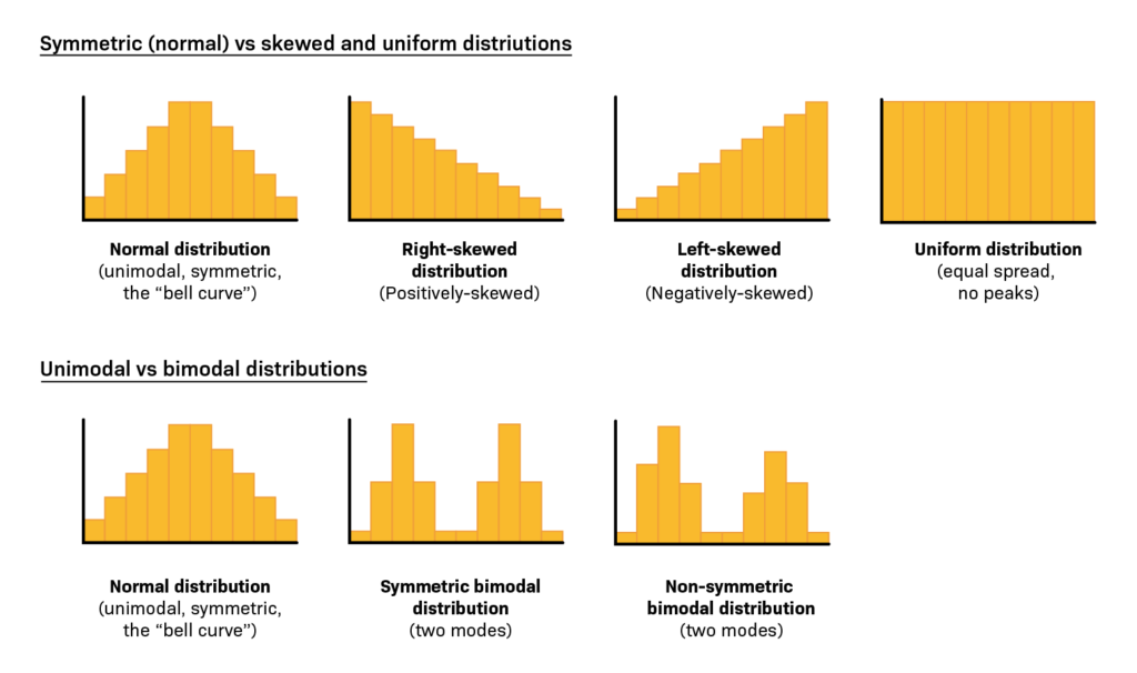
Other Distributions
- Bimodal : It has two distinct peaks, indicating the presence of two separate modes or patterns in the data. This shape suggests that the dataset is a combination of two different underlying distributions.
- Uniform : All values have roughly the same frequency, resulting in a flat, rectangular shape. There are no clear peaks or valleys, and each value has an equal chance of occurrence.
- Multimodal : It has more than two peaks, indicating multiple modes in the dataset. Each peak represents a distinct pattern or subgroup within the data.
- Exponential : It has a rapidly decreasing frequency as values increase. It is characterized by a steep decline in the right tail. The shape is common in datasets where the likelihood of an event decreases exponentially with time.
- Comb: It has alternating high and low frequencies, creating a pattern that resembles the teeth of a comb. This shape suggests periodicity or systematic variation in the data.
5. Normal Q-Q Plot
Furthermore, the Normal Q-Q plot complements the Histogram by providing a visual comparison between the observed data quantiles and the quantiles expected in a normal distribution. By comparing observed quantiles with expected quantiles, researchers gain insights into the conformity of the data to a normal distribution. Clear instructions ensure a seamless incorporation of this method into the normality checking process.
6. Skewness and Kurtosis
It is a statistical measure that quantifies the asymmetry of a probability distribution or a dataset. In the context of data analysis, skewness helps us understand the distribution of values in a dataset and whether it is symmetric or not. The value can be positive, negative, or zero.
- Positive: it indicates that the data distribution is skewed to the right. In other words, the tail on the right side of the distribution is longer or fatter than the left side, and the majority of the data points are concentrated towards the left.
- Negative: Conversely, the data distribution is skewed to the left. The tail on the left side is longer or fatter than the right side, and the majority of data points are concentrated towards the right.
- Zero : A skewness value of zero suggests that the distribution is perfectly symmetrical, with equal tails on both sides.
In summary, skewness provides insights into the shape of the distribution and the relative concentration of data points on either side of the mean.
It is a statistical measure that describes the distribution’s “tailedness” or the sharpness of the peak of a dataset. This helps to identify whether the tails of a distribution contain extreme values. Like skewness, kurtosis can be positive, negative, or zero.
- Positive: The distribution has heavier tails and a sharper peak than the normal distribution. So, It suggests that the dataset has more outliers or extreme values than would be expected in a normal distribution.
- Negative: Conversely, the distribution has lighter tails and a flatter peak than the normal distribution. Therefore, It implies that the dataset has fewer outliers or extreme values than a normal distribution.
- Zero: A kurtosis value of zero, also known as mesokurtic, indicates a distribution with tails and a peak similar to the normal distribution.
In data analysis, For a normal distribution, skewness is close to zero, and kurtosis is around 3 (known as mesokurtic). Deviations from these values may suggest non-normality and guide researchers in choosing appropriate statistical methods.
Example of Normality Test
To provide practical insights, this section will present a hypothetical example illustrating the application of normality tests in SPSS. Through a step-by-step walkthrough, readers will gain a tangible understanding of how to apply the Kolmogorov-Smirnov and Shapiro-Wilk tests to a real-world dataset, reinforcing the theoretical concepts discussed earlier.
Imagine you are a researcher conducting a study on the screen time of a group of individuals. You have collected data on the number of min each participant’s screen time per day. As part of your analysis, you want to assess whether the phone screen time follows a normal distribution. Let’s see how to conduct explore analysis in SPSS.
How to Perform Normality Test in SPSS
Step by Step: Running Normality Analysis in SPSS Statistics
Practicality is paramount, and this section will guide researchers through the step-by-step process of performing a Normality Test in SPSS. From importing the dataset to interpreting the results, this comprehensive guide ensures seamless execution of the normality testing procedure, fostering confidence in the analytical journey.
- STEP: Load Data into SPSS
Commence by launching SPSS and loading your dataset, which should encompass the variables of interest – a categorical independent variable. If your data is not already in SPSS format, you can import it by navigating to File > Open > Data and selecting your data file.
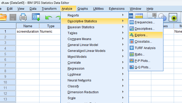
- STEP: Access the Analyze Menu
In the top menu, locate and click on “ Analyze .” Within the “Analyze” menu, navigate to “ Descriptive Statistics ” and choose ” Explore .” Analyze > Descriptive Statistics > Explore
- STEP: Specify Variables
Upon selecting “ Explore ” a dialog box will appear. Choose the variable of interest and move it to the “ Dependent List ” box
- STEP: Define Statistics
Click on the ‘Statistics’ button to include Descriptives, Outliers, and Percentiles.
- STEP: Define the Normality Plot with the Test
Click on the ‘Plot’ button to include visual representations, such as histogram, and stem-and-leaf. Check “ Normality plots with tests ” to obtain a Normal Q-Q plot, Kolmogorov-Smirnov Test, and Shapiro-Wilk test .
6. Final STEP: Generate Normality Test and Chart :
Once you have specified your variables and chosen options, click the “ OK ” button to perform the analysis. SPSS will generate a comprehensive output, including the requested frequency table and chart for your dataset.
Conducting the Normality Test in SPSS provides a robust foundation for understanding the key features of your data. Always ensure that you consult the documentation corresponding to your SPSS version, as steps might slightly differ based on the software version in use. This guide is tailored for SPSS version 25 , and any variations, it’s recommended to refer to the software’s documentation for accurate and updated instructions.
SPSS Output for Normality Test

How to Interpret SPSS Output of Normality Test
Interpreting the output of a normality test is a critical skill for researchers. This section will dissect the SPSS output, explaining how to analyze results from the Kolmogorov-Smirnov and Shapiro-Wilk tests, as well as interpret visual aids like Histograms and Normal Q-Q plots.
- Skewness and Kurtosis: The skewness of approximately 0 suggests a symmetrical distribution, while the negative kurtosis of -0.293 indicates lighter tails compared to a normal distribution.
- Kolmogorov-Smirnov Test: The Kolmogorov-Smirnov test yields a statistic of 0.051 with a p-value of 0.200 (approximately), indicating no significant evidence to reject the null hypothesis of normality.
- Shapiro-Wilk Test: The Shapiro-Wilk test produces a statistic of 0.993 with a p-value of 0.876, providing further support for the assumption of normality.
- Histogram and Normal Q-Q Plot: The Histogram with a central peak, reflects a symmetric distribution, and the Normal Q-Q plot with points closely aligned along a straight line, affirming the approximate normality of the “Screen Time (in min)” variable.
How to Report Results of Normality Analysis in APA
Effective communication of research findings is essential, and this section will guide researchers on how to report the results of normality tests following the guidelines of the American Psychological Association (APA). From structuring sentences to incorporating statistical values, this segment ensures that researchers convey their findings accurately and professionally.

Get Help From SPSSanalysis.com
Embark on a seamless research journey with SPSSAnalysis.com , where our dedicated team provides expert data analysis assistance for students, academicians, and individuals. We ensure your research is elevated with precision. Explore our pages;
- SPSS Data Analysis Help – SPSS Helper ,
- Quantitative Analysis Help ,
- Qualitative Analysis Help ,
- SPSS Dissertation Analysis Help ,
- Dissertation Statistics Help ,
- Statistical Analysis Help ,
- Medical Data Analysis Help .
Connect with us at SPSSAnalysis.com to empower your research endeavors and achieve impactful results. Get a Free Quote Today !
Expert SPSS data analysis assistance available.
Test for normality
In this topic, perform a normality test, types of normality tests, comparison of anderson-darling, kolmogorov-smirnov, and ryan-joiner normality tests.
Choose Stat > Basic Statistics > Normality Test . The test results indicate whether you should reject or fail to reject the null hypothesis that the data come from a normally distributed population. You can do a normality test and produce a normal probability plot in the same analysis. The normality test and probability plot are usually the best tools for judging normality.
The following are types of normality tests that you can use to assess normality.
Anderson-Darling and Kolmogorov-Smirnov tests are based on the empirical distribution function. Ryan-Joiner (similar to Shapiro-Wilk) is based on regression and correlation.
All three tests tend to work well in identifying a distribution as not normal when the distribution is skewed. All three tests are less distinguishing when the underlying distribution is a t-distribution and nonnormality is due to kurtosis. Usually, between the tests based on the empirical distribution function, Anderson-Darling tends to be more effective in detecting departures in the tails of the distribution. Usually, if departure from normality at the tails is the major problem, many statisticians would use Anderson-Darling as the first choice.
If you are checking normality to prepare for a normal capability analysis, the tails are the most critical part of the distribution.
- Minitab.com
- License Portal
- Cookie Settings
You are now leaving support.minitab.com.
Click Continue to proceed to:
Stack Exchange Network
Stack Exchange network consists of 183 Q&A communities including Stack Overflow , the largest, most trusted online community for developers to learn, share their knowledge, and build their careers.
Q&A for work
Connect and share knowledge within a single location that is structured and easy to search.
Normality test: descriptive vs inferential
REVISED ON REQUEST: Is normality test conducted to check sample normality or population normality, most of the times normality test is required to validate the assumptions of parametric test i.e. the population distribution is normal.
ORIGIANLLY POSTED: We have descriptive normality tests like histogram, QQ plot and other graphical methods Skewness and kurtosis numerical measures
Then the inferential methods the Shapiro-Wilk, Anderson-Darling, KS etc
Why would one perform normality test on sample for descriptive results, most of the hypothesis test talks about population being normal which means inferential methods should be used?
Wondering if something is amiss in my understanding.
I am puzzled why and how descriptives are necessary.
- normality-assumption
- 2 $\begingroup$ Could you attempt to clarify your question (by editing the text)? It's really not clear to me what you're asking. $\endgroup$ – Glen_b Commented Dec 13, 2015 at 5:35
- $\begingroup$ When i do histogram on a sample it just represents the sample data normality ie check if the sample is normal or not; where as when i do Shapiro wilk it does test the normality test for the population ie the inferential part....why would i need histogram or simply put why should i care for sample normality when population normality is what should matter $\endgroup$ – noob Commented Dec 13, 2015 at 5:41
- $\begingroup$ The sample is not normal but a sample might be drawn from a population which is normal. $\endgroup$ – Glen_b Commented Dec 13, 2015 at 7:08
- $\begingroup$ Is a normality test - if ever - not done to check the normality of regression residuals? Such a test is not "required", generally choosing the analysis based on such a test invalidates the p-values etc. from the final analysis, some non-normality is not an issue for most methods (esp. If N is large) and more commonly the analsis is chosen up-front based on previous knowledge. $\endgroup$ – Björn Commented Dec 13, 2015 at 7:41
The normality tests are conducted on a sample to test if the sample was drawn from a normal population.
Why would you want 'descriptive' methods like plotting an histogram or a QQ plot? Because sometimes the tests can just be 'wrong' and you have to check visually. Remember that in any goodness of fit test, you don't want to reject $H_0$, but if, for example, you have a very large sample size, the power (the probability of rejecting a false null hypothesis) of the test could be too high and you'll find yourself rejecting $H_0$ with a very high probability (because of small deviations), even if the data is not really that different from the theoretical distribution. If that is the case, a histogram with a QQ Plot may help you in deciding that you can work as if the sample was drawn from a normal distribution.
- $\begingroup$ when i use spss >>explore>>descriptives for normality then histogram , qq , boxplot are suggested by book, where i was wondering does sample data plot showing normality will automatically imply the population normality?? why do literature talk about these ?? $\endgroup$ – noob Commented Dec 13, 2015 at 10:12
- 1 $\begingroup$ @noob Nothing automatically implies population normality. As well explained in this answer, all you have is the sample and a situation in which significance need not mean practical importance. $\endgroup$ – Nick Cox Commented Dec 13, 2015 at 12:40
- $\begingroup$ I can understand that significance is just statistical and might not mean a practical significance . however this shouldn't mean that ...in the realm of hypothesis testing for thesis or other research work ...I can never state that... because inferential statistics might not be robust I abandon them or downplay them...by stating ...descriptives are of practical significance and robust...thus I do inferential if the result is not favorable... I will use descriptives as substitute for inferential... $\endgroup$ – noob Commented Dec 15, 2015 at 17:13
- $\begingroup$ From this can I interpret that when inferential fails to prove we should use descriptives. My further question is why can't we use more robust methods $\endgroup$ – noob Commented Dec 15, 2015 at 17:32
- $\begingroup$ It is not that when inferential fails you should use descriptives. Is just that you can't rely just in one of them $\endgroup$ – toneloy Commented Dec 15, 2015 at 19:32
Your Answer
Sign up or log in, post as a guest.
Required, but never shown
By clicking “Post Your Answer”, you agree to our terms of service and acknowledge you have read our privacy policy .
Not the answer you're looking for? Browse other questions tagged normality-assumption or ask your own question .
- Featured on Meta
- Upcoming initiatives on Stack Overflow and across the Stack Exchange network...
- Announcing a change to the data-dump process
Hot Network Questions
- Why doesn't "I never found the right one" use the present perfect?
- Is this sample LSAT question / answer based in fallacy?
- Let FullSimplify remove a sum-of-squares demoninator
- Travelling from Ireland to Northern Ireland (UK Visa required national)
- Nuda per lusus pectora nostra patent
- How can life which cannot live on the surface of a planet naturally reach the supermajority of the planet's caves?
- Relation between, pre, post, segment and total lengths in Tikz decoration
- 40 minute layover in DFW, changing terminals
- Can a long enough series of numbers in the correct order be all there is to emergent consciousness?
- When I attach a sensitive pdf encrypted by Adobe with a password, and send it through Gmail with password included, does it make any difference?
- Doesn't our awareness of qualia imply the brain is non-deterministic?
- Serre’s comment on Hurwitz: connecting FLT to points of finite order on elliptic curves
- What happens if you're prevented from directing Blast Globes to a target the turn after you activate them?
- Make both colors connected
- How do I write ‘Best friends since 1997’ in latin
- Can Victorian engineers build spacecraft with an Epstein drive?
- Is my connection in Jeddha too short?
- Publishing a paper written in your free time as an unaffiliated author when you are affiliated
- Why is much harder to encrypt emails, compared to web pages?
- Central element of matrix
- What is the meaning of "chabeen" in Conde's "The Gospel According to the New World"?
- How to make sure a payment is actually received and will not bounce, using Paypal, Stripe or online banking respectively?
- Visualising a mapping
- Are 'get something ready' and 'get something going' examples of causative constructions?
Testing Normality in Structural Equation Modeling
When conducting a structural equation model (SEM) or confirmatory factor analysis (CFA) , it is often recommended to test for multivariate normality. Some popular SEM software packages (such as AMOS) assume your variables are continuous and produce the best results when your data are normally distributed. Here we discuss a few options for testing normality in SEM.
First, it is possible to test for multivariate normality using a quantile (Q-Q) or probability (P-P) plot, which can be done though the Analyze > Descriptive Statistics menu in SPSS (see our previous blog on this topic for more details). Similarly, you can conduct a quantile plot of Mahalanobis distances to test for normality (the steps for calculating Mahalanobis distances in SPSS are outlined here ). If you use Intellectus Statistics to conduct your analysis, the Mahalanobis distances method will automatically be performed for you. For all of these methods, a plot is produced, and the points on that plot should follow a relatively straight line. Marked deviations from a straight line suggest that the data are not multivariate normal.
Option 1: User-friendly Software
Transform raw data to written interpreted APA results in seconds.
Option 2: Professional Statistician
Collaborate with a statistician to complete and understand your results.

If you are conducting your analysis in AMOS, the built-in test for normality involves the calculation of Mardia’s coefficient, which is a multivariate measure of kurtosis. AMOS will provide this coefficient and a corresponding “critical value” which can be interpreted as a significance test (a critical value of 1.96 corresponds to a p -value of .05). If Mardia’s coefficient is significant, (i.e., the critical ratio is greater than 1.96 in magnitude) the data may not be normally distributed. However, this significance test on its own is not a practical assessment of normality, especially in SEM. This is because tests such as these are highly sensitive to sample size, with larger sample sizes being more likely to produce significant (non-normal) results. In SEM, where your sample size is expected to be very large, this means that Mardia’s coefficient is almost always guaranteed to be significant. Thus, the significance test on its own does not provide very useful information. In light of this, it is recommended that the significance tests be used in conjunction with descriptive statistics, namely the kurtosis values for individual variables (Stevens, 2009). Kurtosis values greater than 3.00 in magnitude may indicate that a variable is not normally distributed (Westfall & Henning, 2013).
There are many ways to test for normality, and these are just a few of the most popular methods used in support of SEM analysis.
Stevens, J. P. (2009). Applied multivariate statistics for the social sciences (5th ed.). Mahwah, NJ: Routledge Academic.
Westfall, P. H., & Henning, K. S. S. (2013). Texts in statistical science: Understanding advanced statistical methods. Boca Raton, FL: Taylor & Francis.

We work with graduate students every day and know what it takes to get your research approved.
- Address committee feedback
- Roadmap to completion
- Understand your needs and timeframe
- [email protected]
- +1 424 666 28 24
- How it works
- GET YOUR FREE QUOTE
- GET A FREE QUOTE
- Frequently Asked Questions
- Become a Statistician
Reporting Normality Test in SPSS
Looking for Normality Test in SPSS ? Doing it yourself is always cheaper, but it can also be a lot more time-consuming . If you’re not good at SPSS, you can pay someone to do your SPSS task for you.

How to Run Normality Test in SPSS: Explanation Step by Step
From the spss menu, choose analyze – descriptives – explore.

A new window will appear. From the left box, transfer variables Age and Height into Dependent list box. Click Both in the Display box.

Click on Statistics… button. A new window will open. Choose Descriptives. Click Continue, and you will return to the previous box.

Click on Plots… button, New window will open. In the Boxplots box, choose Factor levels together. In the Descriptive box, choose Stem-and-leaf and Normality plots with tests. Click Continue, and you will return to the previous box. Click OK.

The test of normality results will appear in the output window.

How to report a Normality Test results: Explanation Step by Step
How to report case processing summary table in spss output.
The first table is the Case Processing summary table. It shows the number and percent of valid, missing and total cases for variables Age and Height.

How to Report Descriptive Statistics Table in SPSS Output?
The second table shows descriptive statistics for variable Age and Height.

How to Report P-Value of Kolmogorov-Smirnov and Shapiro-Wilk tests of normality Table in SPSS Output?
The third table shows the results of Kolmogorov-Smirnov and Shapiro-Wilk tests of normality (tests statistic, degrees of freedom, p-value). Since we have less than 50 observations (N = 32 < 50), we will interpret the Shapiro-Wilk test results.
Firstly, If p (Sig.) > 0.05, we fail to reject the null hypothesis and conclude that data is normally distributed so we must use parametric tests.
secondly, if the p-value is less than 0.05. Therefore, we must reject the null hypothesis in other words data is not normally distributed. Therefore, We must use nonparametric tests.
In our example, the p-value for age is 0.018 < 0.05. Therefore, we must reject the null hypothesis and conclude that age is not normally distributed.

How to Report Normal Q-Q Plot in SPSS output?
The output also shows the Normal Q-Q Plot for Age and Height.
Firstly, If the data points are close to the diagonal line on the chart so we conclude that data is normally distributed otherwise data set does not show normal distribution.
Lastly, From the chart for age, we can conclude that data points are not close to the diagonal line, we, therefore, conclude that data are not normally distributed.

How to Interpret a Normality Test Results in APA Style?
Shapiro-Wilk test of normality was conducted to determine whether Age and Height data is normally distributed. The results indicate that we must reject the null hypothesis for Age data (p = 0.018) and conclude that data is not normally distributed. Consequently, the results also indicate that we fail to reject the null hypothesis for Height data (p = 0.256) and conclude that data is normally distributed.
Visit our “ How to Run Normality Test in SPSS ” page for more details. Moreover, go to the general page to check Other Reporting Statistical Tests in SPSS . Finally, If you want to watch SPSS videos, Please visit our YouTube Chanel.
GET HELP FROM THE US
There is a lot of statistical software out there, but SPSS is one of the most popular. If you’re a student who needs help with SPSS , there are a few different resources you can turn to. The first is SPSS Video Tutorials . We prepared a page for SPSS Tutor for Beginners . All contents can guide you through Step-by-step SPSS data analysis tutorials and you can see How to Run in Statistical Analysis in SPSS .
The second option is that you can get help from us, we give SPSS help for students with their assignments, dissertation, or research. Doing it yourself is always cheaper, but it can also be a lot more time-consuming. If you’re not the best at SPSS, then this might not be a good idea. It can take days just to figure out how to do some of the easier things in SPSS. So paying someone to do your SPSS will save you a ton of time and make your life a lot easier.
The procedure of the SPSS help service at OnlineSPSS.com is fairly simple. There are three easy-to-follow steps.
1. Click and Get a FREE Quote 2. Make the Payment 3. Get the Solution
Our purpose is to provide quick, reliable, and understandable information about SPSS data analysis to our clients.

- Affiliated Shengjing Hospital of China Medical University
Which part is the best for normality test results in the paper?
Most recent answer.

Top contributors to discussions in this field

- Rutgers, The State University of New Jersey

- EMINENT BIOSCIENCES

- Mississippi State University (Emeritus)

- North-West University
- University of Nevada, Las Vegas
Get help with your research
Join ResearchGate to ask questions, get input, and advance your work.
All replies (5)
Similar questions and discussions
- Asked 8 December 2020

- Asked 3 January 2015
- Asked 10 March 2021
- Asked 4 July 2019

- Asked 22 May 2019

- Asked 1 June 2022

- Asked 12 November 2019

- Asked 23 June 2018

- Asked 24 October 2017

Related Publications

- Recruit researchers
- Join for free
- Login Email Tip: Most researchers use their institutional email address as their ResearchGate login Password Forgot password? Keep me logged in Log in or Continue with Google Welcome back! Please log in. Email · Hint Tip: Most researchers use their institutional email address as their ResearchGate login Password Forgot password? Keep me logged in Log in or Continue with Google No account? Sign up
IMAGES
VIDEO
COMMENTS
Descriptive statistics are an important part of biomedical research which is used to describe the basic features of the data in the study. They provide simple summaries about the sample and the measures. Measures of the central tendency and dispersion are used to describe the quantitative data. For the continuous data, test of the normality is ...
A normality test determines whether a sample data has been drawn from a normally distributed population. It is generally performed to verify whether the data involved in the research have a normal distribution. Many statistical procedures such as correlation, regression, t-tests, and ANOVA, namely parametric tests, are based on the normal ...
The Shapiro-Wilk test is based on the correlation between the data and the corresponding normal scores and provides better power than the K-S test even after the Lilliefors correction . Power is the most frequent measure of the value of a test for normality—the ability to detect whether a sample comes from a non-normal distribution ( 11 ).
Normality Tests for Statistical Analysis: A Guide for Non-Statisticians. December 2012. International Journal of Endocrinology and Metabolism 10 (2):486-489. DOI: 10.5812/ijem.3505. Source. PubMed ...
A Brief Review of Tests for Normality. American Journal of Theoretical and Applied Statistics. V ol. 5, No. 1, 2016, pp. 5-12. doi: 10.11648/j.ajtas.20160501.12. Abstract: In statistics it is ...
The starting po int for identifying normality is the histogram, which is simply a frequency bar -. plot (either absolute or relative) of the data. In histograms of no rmally-distributed data, the ...
The most common analytical tests to check data for normal distribution are the: Kolmogorov-Smirnov Test. Shapiro-Wilk Test. Anderson-Darling Test. For graphical verification, either a histogram or, better, the Q-Q plot is used. Q-Q stands for quantile-quantile plot, where the actually observed distribution is compared with the theoretically ...
A fairly simple test that requires only the sample standard deviation and the data range. Should not be confused with the Shapiro-Wilk test. Based on the q statistic, which is the 'studentized' (meaning t distribution) range, or the range expressed in standard deviation units. where.
The assumptions of normality and homogeneity of variance were assessed. Normality. A Shapiro-Wilk test was conducted to determine whether MiniCog could have been produced by a normal distribution (Razali & Wah, 2011). The results of the Shapiro-Wilk test were significant, W = 0.94, p = .007. These results suggest that MiniCog is unlikely to ...
For these techniques, it is good practice to examine the data to confirm that the assumption of normality is tenable. With that in mind, here are three simple ways to test interval-scale data or ratio-scale data for normality. Check descriptive statistics. Generate a histogram. Conduct a chi-square test.
A Normal Distribution Test, as the name implies, is a statistical method employed to determine if a dataset follows a normal distribution. The assumption of normality is fundamental in various statistical analyses, such as t-tests and ANOVA. In the context of SPSS, researchers utilize tests like the Kolmogorov-Smirnov test and Shapiro-Wilk test ...
r the researchers to show normality by using skewness and kurtosis values. Based on the criteria chos. n to check normality it is decided to use parametric or nonparametric. tests. If the criterion is changed, the test to be chosen might also change. For example, if one use "skewness smaller than 1" instead of "z-.
the case when the reviewer requests the normality check or test in the review process of a thesis, the normality test is carried out to correct the contents of the submitted papers. However, when this lack of the normality check or test goes unnoticed, the results are frequently presented without a normality test. If the statistical analysis method
Example of a. Normality Test. A scientist for a company that manufactures processed food wants to assess the percentage of fat in the company's bottled sauce. The advertised percentage is 15%. The scientist measures the percentage of fat in 20 random samples. The scientist wants to verify the assumption of normality before performing a ...
As a review of hypothesis testing in a second semester undergrad course in statistics, we develop, in class, the test of normality due to Filliben (1975), using the correlation coefficient of the QQ plot. The development starts with the data set of MacDonald and Schwing (1973) demonstrating a variety of histogram and QQ plot shapes.
Ryan-Joiner normality test. This test assesses normality by calculating the correlation between your data and the normal scores of your data. If the correlation coefficient is near 1, the population is likely to be normal. The Ryan-Joiner statistic assesses the strength of this correlation; if it is less than the appropriate critical value, you ...
Thesis. Dec 2021; Yifan Zhang ... The results of the data normality test calculation used the Kolmogorov Smirnov test at a significance level of 0.05, showing a significance value> 0.05, so that ...
REVISED ON REQUEST: Is normality test conducted to check sample normality or population normality, most of the times normality test is required to validate the assumptions of parametric test i.e. the population distribution is normal. ORIGIANLLY POSTED: We have descriptive normality tests like histogram, QQ plot and other graphical methods ...
Simple back-of-the-envelope test takes the sample maximum and minimum and computes their z-score, or more properly t-statistic (number of sample standard deviations that a sample is above or below the sample mean), and compares it to the 68-95-99.7 rule: if one has a 3σ event (properly, a 3s event) and substantially fewer than 300 samples, or a 4s event and substantially fewer than 15,000 ...
If you are conducting your analysis in AMOS, the built-in test for normality involves the calculation of Mardia's coefficient, which is a multivariate measure of kurtosis. AMOS will provide this coefficient and a corresponding "critical value" which can be interpreted as a significance test (a critical value of 1.96 corresponds to a p ...
The procedure of the SPSS help service at OnlineSPSS.com is fairly simple. There are three easy-to-follow steps. 1. Click and Get a FREE Quote. 2. Make the Payment. 3. Get the Solution. Our purpose is to provide quick, reliable, and understandable information about SPSS data analysis to our clients.
It is known as JB Test in short. This test gives the value of 2 for df = 2. to test the normality of d istribution. If the 2 obtained by this test is smaller than table value. of 2 for df = 2 at 0 ...
Pre-test is done on Thursday, 4 March, 2016. For pre-test the researcher give the students hortatory exposition prompt. Students are asked to make an essay about hortatory exposition text based on the instruction (prompt). To analyze the pre-test result, the researcher oriented on writing scoring rubric. 2. Post-test
If you just inspected a quantile-quantile plot of model residuals to a normal distribution, then no p-value applies. Good luck with your work. Thank you David Morse . And yes, that's would be the ...