Thank you for visiting nature.com. You are using a browser version with limited support for CSS. To obtain the best experience, we recommend you use a more up to date browser (or turn off compatibility mode in Internet Explorer). In the meantime, to ensure continued support, we are displaying the site without styles and JavaScript.
- View all journals
- Explore content
- About the journal
- Publish with us
- Sign up for alerts
- Published: 29 May 2014
Points of significance

Designing comparative experiments
- Martin Krzywinski 1 &
- Naomi Altman 2
Nature Methods volume 11 , pages 597–598 ( 2014 ) Cite this article
48k Accesses
14 Citations
8 Altmetric
Metrics details
- Research data
- Statistical methods
Good experimental designs limit the impact of variability and reduce sample-size requirements.
You have full access to this article via your institution.
In a typical experiment, the effect of different conditions on a biological system is compared. Experimental design is used to identify data-collection schemes that achieve sensitivity and specificity requirements despite biological and technical variability, while keeping time and resource costs low. In the next series of columns we will use statistical concepts introduced so far and discuss design, analysis and reporting in common experimental scenarios.
In experimental design, the researcher-controlled independent variables whose effects are being studied (e.g., growth medium, drug and exposure to light) are called factors. A level is a subdivision of the factor and measures the type (if categorical) or amount (if continuous) of the factor. The goal of the design is to determine the effect and interplay of the factors on the response variable (e.g., cell size). An experiment that considers all combinations of N factors, each with n i levels, is a factorial design of type n 1 × n 2 × ... × n N . For example, a 3 × 4 design has two factors with three and four levels each and examines all 12 combinations of factor levels. We will review statistical methods in the context of a simple experiment to introduce concepts that apply to more complex designs.
Suppose that we wish to measure the cellular response to two different treatments, A and B, measured by fluorescence of an aliquot of cells. This is a single factor (treatment) design with three levels (untreated, A and B). We will assume that the fluorescence (in arbitrary units) of an aliquot of untreated cells has a normal distribution with μ = 10 and that real effect sizes of treatments A and B are d A = 0.6 and d B = 1 (A increases response by 6% to 10.6 and B by 10% to 11). To simulate variability owing to biological variation and measurement uncertainty (e.g., in the number of cells in an aliquot), we will use σ = 1 for the distributions. For all tests and calculations we use α = 0.05.
We start by assigning samples of cell aliquots to each level ( Fig. 1a ). To improve the precision (and power) in measuring the mean of the response, more than one aliquot is needed 1 . One sample will be a control (considered a level) to establish the baseline response, and capture biological and technical variability. The other two samples will be used to measure response to each treatment. Before we can carry out the experiment, we need to decide on the sample size.

( a ) Two treated samples (A and B) with n = 17 are compared to a control (C) with n = 17 and to each other using two-sample t -tests. ( b ) Simulated means and P values for samples in a . Values are drawn from normal populations with σ = 1 and mean response of 10 (C), 10.6 (A) and 11 (B). ( c ) The preferred reporting method of results shown in b , illustrating difference in means with CIs, P values and effect size, d . All error bars show 95% CI.
We can fall back to our discussion about power 1 to suggest n . How large an effect size ( d ) do we wish to detect and at what sensitivity? Arbitrarily small effects can be detected with large enough sample size, but this makes for a very expensive experiment. We will need to balance our decision based on what we consider to be a biologically meaningful response and the resources at our disposal. If we are satisfied with an 80% chance (the lowest power we should accept) of detecting a 10% change in response, which corresponds to the real effect of treatment B ( d B = 1), the two-sample t -test requires n = 17. At this n value, the power to detect d A = 0.6 is 40%. Power calculations are easily computed with software; typically inputs are the difference in means (Δ μ ), standard deviation estimate ( σ ), α and the number of tails (we recommend always using two-tailed calculations).
Based on the design in Figure 1a , we show the simulated samples means and their 95% confidence interval (CI) in Figure 1b . The 95% CI captures the mean of the population 95% of the time; we recommend using it to report precision. Our results show a significant difference between B and control (referred to as B/C, P = 0.009) but not for A/C ( P = 0.18). Paradoxically, testing B/A does not return a significant outcome ( P = 0.15). Whenever we perform more than one test we should adjust the P values 2 . As we only have three tests, the adjusted B/C P value is still significant, P ′ = 3 P = 0.028. Although commonly used, the format used in Figure 1b is inappropriate for reporting our results: sample means, their uncertainty and P values alone do not present the full picture.
A more complete presentation of the results ( Fig. 1c ) combines the magnitude with uncertainty (as CI) in the difference in means. The effect size, d , defined as the difference in means in units of pooled standard deviation, expresses this combination of measurement and precision in a single value. Data in Figure 1c also explain better that the difference between a significant result (B/C, P = 0.009) and a nonsignificant result (A/C, P = 0.18) is not always significant (B/A, P = 0.15) 3 . Significance itself is a hard boundary at P = α , and two arbitrarily close results may straddle it. Thus, neither significance itself nor differences in significance status should ever be used to conclude anything about the magnitude of the underlying differences, which may be very small and not biologically relevant.
CIs explicitly show how close we are to making a positive inference and help assess the benefit of collecting more data. For example, the CIs of A/C and B/C closely overlap, which suggests that at our sample size we cannot reliably distinguish between the response to A and B ( Fig. 1c ). Furthermore, given that the CI of A/C just barely crosses zero, it is possible that A has a real effect that our test failed to detect. More information about our ability to detect an effect can be obtained from a post hoc power analysis, which assumes that the observed effect is the same as the real effect (normally unknown), and uses the observed difference in means and pooled variance. For A/C, the difference in means is 0.48 and the pooled s.d. ( s p ) = 1.03, which yields a post hoc power of 27%; we have little power to detect this difference. Other than increasing sample size, how could we improve our chances of detecting the effect of A?
Our ability to detect the effect of A is limited by variability in the difference between A and C, which has two random components. If we measure the same aliquot twice, we expect variability owing to technical variation inherent in our laboratory equipment and variability of the sample over time ( Fig. 2a ). This is called within-subject variation, σ wit . If we measure two different aliquots with the same factor level, we also expect biological variation, called between-subject variation, σ bet , in addition to the technical variation ( Fig. 2b ). Typically there is more biological than technical variability ( σ bet > σ wit ). In an unpaired design, the use of different aliquots adds both σ wit and σ bet to the measured difference ( Fig. 2c ). In a paired design, which uses the paired t -test 4 , the same aliquot is used and the impact of biological variation ( σ bet ) is mitigated ( Fig. 2c ). If differences in aliquots ( σ bet ) are appreciable, variance is markedly reduced (to within-subject variation) and the paired test has higher power.

( a ) Limits of measurement and technical precision contribute to σ wit (gray circle) observed when the same aliquot is measured more than once. This variability is assumed to be the same in the untreated and treated condition, with effect d on aliquot x and y . ( b ) Biological variation gives rise to σ bet (green circle). ( c ) Paired design uses the same aliquot for both measurements, mitigating between-subject variation.
The link between σ bet and σ wit can be illustrated by an experiment to evaluate a weight-loss diet in which a control group eats normally and a treatment group follows the diet. A comparison of the mean weight after a month is confounded by the initial weights of the subjects in each group. If instead we focus on the change in weight, we remove much of the subject variability owing to the initial weight.
If we write the total variance as σ 2 = σ wit 2 + σ bet 2 , then the variance of the observed quantity in Figure 2c is 2 σ 2 for the unpaired design but 2 σ 2 (1 – ρ ) for the paired design, where ρ = σ bet 2 / σ 2 is the correlation coefficient (intraclass correlation). The relative difference is captured by ρ of two measurements on the same aliquot, which must be included because the measurements are no longer independent. If we ignore ρ in our analysis, we will overestimate the variance and obtain overly conservative P values and CIs. In the case where there is no additional variation between aliquots, there is no benefit to using the same aliquot: measurements on the same aliquot are uncorrelated ( ρ = 0) and variance of the paired test is the same as the variance of the unpaired. In contrast, if there is no variation in measurements on the same aliquot except for the treatment effect ( σ wit = 0), we have perfect correlation ( ρ = 1). Now, the difference measurement derived from the same aliquot removes all the noise; in fact, a single pair of aliquots suffices for an exact inference. Practically, both sources of variation are present, and it is their relative size—reflected in ρ —that determines the benefit of using the paired t-test.
We can see the improved sensitivity of the paired design ( Fig. 3a ) in decreased P values for the effects of A and B ( Fig. 3b versus Fig. 1b ). With the between-subject variance mitigated, we now detect an effect for A ( P = 0.013) and an even lower P value for B ( P = 0.0002) ( Fig. 3b ). Testing the difference between ΔA and ΔB requires the two-sample t -test because we are testing different aliquots, and this still does not produce a significant result ( P = 0.18). When reporting paired-test results, sample means ( Fig. 3b ) should never be shown; instead, the mean difference and confidence interval should be shown ( Fig. 3c ). The reason for this comes from our discussion above: the benefit of pairing comes from reduced variance because ρ > 0, something that cannot be gleaned from Figure 3b . We illustrate this in Figure 3c with two different sample simulations with same sample mean and variance but different correlation, achieved by changing the relative amount of σ bet 2 and σ wit 2 . When the component of biological variance is increased, ρ is increased from 0.5 to 0.8, total variance in difference in means drops and the test becomes more sensitive, reflected by the narrower CIs. We are now more certain that A has a real effect and have more reason to believe that the effects of A and B are different, evidenced by the lower P value for ΔB/ΔA from the two-sample t -test (0.06 versus 0.18; Fig. 3c ). As before, P values should be adjusted with multiple-test correction.

( a ) The same n = 17 sample is used to measure the difference between treatment and background (ΔA = A after − A before , ΔB = B after − B before ), analyzed with the paired t -test. Two-sample t -test is used to compare the difference between responses (ΔB versus ΔA). ( b ) Simulated sample means and P values for measurements and comparisons in a . ( c ) Mean difference, CIs and P values for two variance scenarios, σ bet 2 / σ wit 2 of 1 and 4, corresponding to ρ of 0.5 and 0.8. Total variance was fixed: σ bet 2 + σ wit 2 = 1. All error bars show 95% CI.
The paired design is a more efficient experiment. Fewer aliquots are needed: 34 instead of 51, although now 68 fluorescence measurements need to be taken instead of 51. If we assume σ wit = σ bet ( ρ = 0.5; Fig. 3c ), we can expect the paired design to have a power of 97%. This power increase is highly contingent on the value of ρ . If σ wit is appreciably larger than σ bet (i.e., ρ is small), the power of the paired test can be lower than for the two-sample variant. This is because total variance remains relatively unchanged (2 σ 2 (1 – ρ ) ≈ 2 σ 2 ) while the critical value of the test statistic can be markedly larger (particularly for small samples) because the number of degrees of freedom is now n – 1 instead of 2( n – 1). If the ratio of σ bet 2 to σ wit 2 is 1:4 ( ρ = 0.2), the paired test power drops from 97% to 86%.
To analyze experimental designs that have more than two levels, or additional factors, a method called analysis of variance is used. This generalizes the t -test for comparing three or more levels while maintaining better power than comparing all sets of two levels. Experiments with two or more levels will be our next topic.
Krzywinski, M.I. & Altman, N. Nat. Methods 10 , 1139–1140 (2013).
Article CAS Google Scholar
Krzywinski, M.I. & Altman, N. Nat. Methods 11 , 355–356 (2014).
Gelman, A. & Stern, H. Am. Stat. 60 , 328–331 (2006).
Article Google Scholar
Krzywinski, M.I. & Altman, N. Nat. Methods 11 , 215–216 (2014).
Download references
Author information
Authors and affiliations.
Martin Krzywinski is a staff scientist at Canada's Michael Smith Genome Sciences Centre.,
- Martin Krzywinski
Naomi Altman is a Professor of Statistics at The Pennsylvania State University.,
- Naomi Altman
You can also search for this author in PubMed Google Scholar
Ethics declarations
Competing interests.
The authors declare no competing financial interests.
Rights and permissions
Reprints and permissions
About this article
Cite this article.
Krzywinski, M., Altman, N. Designing comparative experiments. Nat Methods 11 , 597–598 (2014). https://doi.org/10.1038/nmeth.2974
Download citation
Published : 29 May 2014
Issue Date : June 2014
DOI : https://doi.org/10.1038/nmeth.2974
Share this article
Anyone you share the following link with will be able to read this content:
Sorry, a shareable link is not currently available for this article.
Provided by the Springer Nature SharedIt content-sharing initiative
This article is cited by
Sources of variation.
Nature Methods (2015)
ETD Outperforms CID and HCD in the Analysis of the Ubiquitylated Proteome
- Tanya R. Porras-Yakushi
- Michael J. Sweredoski
Journal of the American Society for Mass Spectrometry (2015)
Analysis of variance and blocking
Nature Methods (2014)
Nested designs
- Paul Blainey
Quick links
- Explore articles by subject
- Guide to authors
- Editorial policies
Sign up for the Nature Briefing newsletter — what matters in science, free to your inbox daily.

Warning: The NCBI web site requires JavaScript to function. more...

An official website of the United States government
The .gov means it's official. Federal government websites often end in .gov or .mil. Before sharing sensitive information, make sure you're on a federal government site.
The site is secure. The https:// ensures that you are connecting to the official website and that any information you provide is encrypted and transmitted securely.
- Publications
- Account settings
- Browse Titles
NCBI Bookshelf. A service of the National Library of Medicine, National Institutes of Health.
Velentgas P, Dreyer NA, Nourjah P, et al., editors. Developing a Protocol for Observational Comparative Effectiveness Research: A User's Guide. Rockville (MD): Agency for Healthcare Research and Quality (US); 2013 Jan.

Developing a Protocol for Observational Comparative Effectiveness Research: A User's Guide.
- Hardcopy Version at Agency for Healthcare Research and Quality
Chapter 2 Study Design Considerations
Til Stürmer , MD, MPH, PhD and M. Alan Brookhart , PhD.
The choice of study design often has profound consequences for the causal interpretation of study results. The objective of this chapter is to provide an overview of various study design options for nonexperimental comparative effectiveness research (CER), with their relative advantages and limitations, and to provide information to guide the selection of an appropriate study design for a research question of interest. We begin the chapter by reviewing the potential for bias in nonexperimental studies and the central assumption needed for nonexperimental CER—that treatment groups compared have the same underlying risk for the outcome within subgroups definable by measured covariates (i.e., that there is no unmeasured confounding). We then describe commonly used cohort and case-control study designs, along with other designs relevant to CER such as case-cohort designs (selecting a random sample of the cohort and all cases), case-crossover designs (using prior exposure history of cases as their own controls), case–time controlled designs (dividing the case-crossover odds ratio by the equivalent odds ratio estimated in controls to account for calendar time trends), and self-controlled case series (estimating the immediate effect of treatment in those treated at least once). Selecting the appropriate data source, patient population, inclusion/exclusion criteria, and comparators are discussed as critical design considerations. We also describe the employment of a “new user” design, which allows adjustment for confounding at treatment initiation without the concern of mixing confounding with selection bias during followup, and discuss the means of recognizing and avoiding immortal-time bias, which is introduced by defining the exposure during the followup time versus the time prior to followup. The chapter concludes with a checklist for the development of the study design section of a CER protocol, emphasizing the provision of a rationale for study design selection and the need for clear definitions of inclusion/exclusion criteria, exposures (treatments), outcomes, confounders, and start of followup or risk period.
- Introduction
The objective of this chapter is to provide an overview of various study design options for nonexperimental comparative effectiveness research (CER), with their relative advantages and limitations. Of the multitude of epidemiologic design options, we will focus on observational designs that compare two or more treatment options with respect to an outcome of interest in which treatments are not assigned by the investigator but according to routine medical practice. We will not cover experimental or quasi-experimental designs, such as interrupted time series, 1 designed delays, 2 cluster randomized trials, individually randomized trials, pragmatic trials, or adaptive trials. These designs also have important roles in CER; however, the focus of this guide is on nonexperimental approaches that directly compare treatment options.
The choice of study design often has profound consequences for the causal interpretation of study results that are irreversible in many settings. Study design decisions must therefore be considered even more carefully than analytic decisions, which often can be changed and adapted at later stages of the research project. Those unfamiliar with nonexperimental design options are thus strongly encouraged to involve experts in the design of nonexperimental treatment comparisons, such as epidemiologists, especially ones familiar with comparing medical treatments (e.g., pharmacoepidemiologists), during the planning stage of a CER study and throughout the project. In the planning stage of a CER study, researchers need to determine whether the research question should be studied using nonexperimental or experimental methods (or a combination thereof, e.g., two-stage RCTs). 3 - 4 Feasibility may determine whether an experimental or a nonexperimental design is most suitable, and situations may arise where neither approach is feasible.
- Issues of Bias in Observational CER
In observational CER, the exposures or treatments are not assigned by the investigator but rather by mechanisms of routine practice. Although the investigator can (and should) speculate on the treatment assignment process or mechanism, the actual process will be unknown to the investigator. The nonrandom nature of treatment assignment leads to the major challenge in nonexperimental CER studies, that of ensuring internal validity. Internal validity is defined as the absence of bias; biases may be broadly classified as selection bias, information bias, and confounding bias. Epidemiology has advanced our thinking about these biases for more than 100 years, and many papers have been published describing the underlying concepts and approaches to bias reduction. For a comprehensive description and definition of these biases, we suggest the book Modern Epidemiology. 5 Ensuring a study's internal validity is a prerequisite for its external validity or generalizability The limited generalizability of findings from randomized controlled trials (RCTs), such as to older adults, patients with comorbidities or comedications, is one of the major drivers for the conduct of nonexperimental CER.
The central assumption needed for nonexperimental CER is that the treatment groups compared have the same underlying risk for the outcome within subgroups definable by measured covariates. Until recently, this “no unmeasured confounding” assumption was deemed plausible only for unintended (usually adverse) effects of medical interventions, that is, for safety studies. The assumption was considered to be less plausible for intended effects of medical interventions (effectiveness) because of intractable confounding by indication. 6 - 7 Confounding by indication leads to higher propensity for treatment or more intensive treatment in those with the most severe disease. A typical example would be a study on the effects of beta-agonists on asthma mortality in patients with asthma. The association between treatment (intensity) with beta-agonists and asthma mortality would be confounded by asthma severity. The direction of the confounding by asthma severity would tend to make the drug look bad (as if it is “causing” mortality). The study design challenge in this example would not be the confounding itself, but the fact that it is hard to control for asthma severity because it is difficult to measure precisely. Confounding by frailty has been identified as another potential bias when assessing preventive treatments in population-based studies, particularly those among older adults. 8 - 11 Because frail persons (those close to death) are less likely to be treated with a multitude of preventive treatments, 8 frailty would lead to confounding, which would bias the association between preventive treatments and outcomes associated with frailty (e.g., mortality). Since the bias would be that the untreated cohort has a higher mortality irrespective of the treatment, this would make the drug's effectiveness look too good. Here again the crux of the problem is that frailty is hard to control for because it is difficult to measure.
- Basic Epidemiologic Study Designs
The general principle of epidemiologic study designs is to compare the distribution of the outcome of interest in groups characterized by the exposure/treatment/intervention of interest. The association between the exposure and outcome is then assessed using measures of association. The causal interpretation of these associations is dependent on additional assumptions, most notably that the risk for the outcome is the same in all treatment groups compared (before they receive the respective treatments), also called exchangeability. 12 - 13 Additional assumptions for a causal interpretation, starting with the Hill criteria, 14 are beyond the scope of this chapter, although most of these are relevant to many CER settings. For situations where treatment effects are heterogeneous, see chapter 3 .
The basic epidemiologic study designs are usually defined by whether study participants are sampled based on their exposure or outcome of interest. In a cross-sectional study, participants are sampled independent of exposure and outcome, and prevalence of exposure and outcome are assessed at the same point in time. In cohort studies, participants are sampled according to their exposures and followed over time for the incidence of outcomes. In case-control studies, cases and controls are sampled based on the outcome of interest, and the prevalence of exposure in these two groups is then compared. Because the cross-sectional study design usually does not allow the investigator to define whether the exposure preceded the outcome, one of the prerequisites for a causal interpretation, we will focus on cohort and case-control studies as well as some more advanced designs with specific relevance to CER.
Definitions of some common epidemiologic terms are presented in Table 2.1 . Given the space constraints and the intended audience, these definitions do not capture all nuances.
Definition of epidemiologic terms.
Cohort Study Design
Description.
Cohorts are defined by their exposure at a certain point in time (baseline date) and are followed over time after baseline for the occurrence of the outcome. For the usual study of first occurrence of outcomes, cohort members with the outcome prevalent at baseline need to be excluded. Cohort entry (baseline) is ideally defined by a meaningful event (e.g., initiation of treatment; see the section on new user design) rather than convenience (prevalence of treatment), although this may not always be feasible or desirable.
The main advantage of the cohort design is that it has a clear timeline separating potential confounders from the exposure and the exposure from the outcome. Cohorts allow the estimation of actual incidence (risk or rate) in all treatment groups and thus the estimation of risk or rate differences. Cohort studies allow investigators to assess multiple outcomes from given treatments. The cohort design is also easy to conceptualize and readily compared to the RCT, a design with which most medical researchers are very familiar.
Limitations
If participants need to be recruited and followed over time for the incidence of the outcome, the cohort design quickly becomes inefficient when the incidence of the outcome is low. This limitation has led to the widespread use of case-control designs (see below) in pharmacoepidemiologic studies using large automated databases. With the IT revolution over the past 10 years, lack of efficiency is rarely, if ever, a reason not to implement a cohort study even in the largest health care databases if all the data have already been collected.
Important Considerations
Patients can only be excluded from the cohort based on information available at start of followup (baseline). Any exclusion of cohort members based on information accruing during followup, including treatment changes, has a strong potential to introduce bias. The idea to have a “clean” treatment group usually introduces selection bias, such as by removing the sickest, those with treatment failure, or those with adverse events, from the cohort. The fundamental principle of the cohort is the enumeration of people at baseline (based on inclusion and exclusion criteria) and reporting losses to followup for everyone enrolled at baseline.
Clinical researchers may also be tempted to assess the treatments during the same time period the outcome is assessed (i.e., during followup) instead of prior to followup. Another fundamental of the cohort design is, however, that the exposure is assessed prior to the assessment of the outcome, thus limiting the potential for incorrect causal inference if the outcome also influences the likelihood of exposure. This general principle also applies to time-varying treatments for which the followup time needs to start anew after treatment changes rather than from baseline.
Cadarette et al. 15 employed a cohort design to investigate the comparative effectiveness of four alternative treatments to prevent osteoporotic fractures. The four cohorts were defined by the initiation of the four respective treatments (the baseline date). Cohorts were followed from baseline to the first occurrence of a fracture at various sites. To minimize bias, statistical analyses adjusted for risk factors for fractures assessed at baseline. As discussed the cohort design provided a clear timeline, differentiating exposure from potential confounders and the outcomes.
Case-Control Study Design
Nested within an underlying cohort, the case-control design identifies all incident cases that develop the outcome of interest and compares their exposure history with the exposure history of controls sampled at random from everyone within the cohort still at risk for developing the outcome of interest. Given proper sampling of controls from the risk set, the estimation of the odds ratio in a case-control study is a computationally more efficient way to estimate the otherwise identical incidence rate ratio in the underlying cohort.
The oversampling of persons with the outcome increases efficiency compared with the full underlying cohort. As outlined above, this efficiency advantage is of minor importance in many CER settings. Efficiency is of major importance, however, if additional data (e.g., blood levels, biologic materials, validation data) need to be collected. It is straightforward to assess multiple exposures, although this will quickly become very complicated when implementing a new user design.
The case-control study is difficult to conceptualize. Some researchers do not understand, for example, that matching does not control for confounding in a case-control study, whereas it does in a cohort study. 16 Unless additional information from the underlying cohort is available, risk or rate differences cannot be estimated from case-control studies. Because the timing between potential confounders and the treatments is often not taken into account, current implementations of the case-control design assessing confounders at the index date rather than prior to treatment initiation will be biased when controlling for covariates that may be affected by prior treatment. Thus, implementing a new user design with proper definition of confounders will often be difficult, although not impossible. If information on treatments needs to be obtained retrospectively, such as from an interview with study participants identified as cases and controls, there is the potential that treatments will be assessed differently for cases and controls, which will lead to bias (often referred to as recall bias).
Controls need to be sampled from the “risk set,” i.e., all patients from the underlying cohort who remain at risk for the outcome at the time a case occurs. Sampling of controls from all those who enter the cohort (i.e., at baseline) may lead to biased estimates of treatment effects if treatments are associated with loss to followup or mortality. Matching on confounders can improve the efficiency of estimation of treatment effects, but does not control for confounding in case-control studies. Matching should only be considered for strong risk factors for the outcome; however, the often small gain in efficiency must be weighed against the loss of the ability to estimate the effect of the matching variable on the outcome (which could, for example, be used as a positive control to show content validity of an outcome definition). 17 Matching on factors strongly associated with treatment often reduces efficiency of case-control studies (overmatching). Generally speaking, matching should not routinely be performed in case-control studies but be carefully considered ideally after some study of the expected efficiency gains. 16 , 18
Martinez et al. 19 conducted a case-control study employing a new user design. The investigators compared venlafaxine and other antidepressants and risk of sudden cardiac death or near death. An existing cohort of new users of antidepressants was identified. (“New users” were defined as subjects without a prescription for the medication in the year prior to cohort entry). Nested within the underlying cohort, cases and up to 30 randomly selected matched controls were identified. Potential controls were assigned an “index date” corresponding to the same followup time to event as the matched case. Controls were only sampled from the “risk set.” That is, controls had to be at risk for the outcome on their index date, thus ensuring that bias was not introduced via the sampling scheme.
Case-Cohort Study Design
In the case-cohort design, cohorts are defined as in a cohort study, and all cohort members are followed for the incidence of the outcomes. Additional information required for analysis (e.g., blood levels, biologic materials for genetic analyses) is collected for a random sample of the cohort and for all cases. (Note that the random sample may contain cases.) This sampling needs to be accounted for in the analysis, 20 but otherwise this design offers all the advantages and possibilities of a cohort study. The case-cohort design is intended to increase efficiency compared with the nested case-control design when selecting participants for whom additional information needs to be collected or when studying more than one outcome.
- Other Epidemiological Study Designs Relevant to CER
Case-Crossover Design
Faced with the problem of selection of adequate controls in a case-control study of triggers of myocardial infarction, Maclure proposed to use prior exposure history of cases as their own controls. 21 For this study design, only patients with the outcome (cases) who have discrepant exposures during the case and the control period contribute information. A feature of this design is that it is self-controlled which removes the confounding effect of any characteristic of subjects that is stable over time (e.g., genetics). For CER, the latter property of the case-crossover design is a major advantage, because measures of stable confounding factors (to address confounding) are not needed. The former property or initial reason to develop the case-crossover design, that is, its ability to assess triggers of (or immediate, reversible effects of, e.g., treatments on) outcomes may also have specific advantages for CER. The case-crossover design is thought to be appropriate for studying acute effects of transient exposures.
While the case-crossover design has been developed to compare exposed with unexposed periods rather than compare two active treatment periods, it may still be valuable for certain CER settings. This would include situations in which patients switch between two similar treatments without stopping treatment. Often such switching would be triggered by health events, which could cause within-person confounding, but when the causes of switching are unrelated to health events (e.g., due to changes in health plan drug coverage), within-person estimates of effect from crossover designs could be unbiased. More work is needed to evaluate the potential to implement the case-crossover design in the presence of treatment gaps (neither treatment) or of more than two treatments that need to be compared.
Exactly as in a case-control study, the first step is to identify all cases with the outcome and assess the prevalence of exposure during a brief time window before the outcome occurred. Instead of sampling controls, we create a separate observation for each case that contains all the same variables except for the exposure, which is defined for a different time period. This “control” time period has the same length as the case period and needs to be carefully chosen to take, for example, seasonality of exposures into account. The dataset is then analyzed as an individually matched case-control study.
The lack of need to select controls, the ability to assess short-term reversible effects, the ability to inform about the time window for this effect using various intervals to define treatment, and the control for all, even unmeasured factors that are stable over time are the major advantages of the case-crossover design. The design can also be easily added to any case-control study with little (if any) cost.
Because only cases with discrepant exposure histories contribute information to the analysis, the case-crossover design is often not very efficient. This may not be a major issue if the design is used in addition to the full case-control design. While the design avoids confounding by factors that are stable over time, it can still be confounded by factors that vary over time. The possibility of time-varying conditions leading to changes in treatment and increasing the risk for the outcome (i.e., confounding by indication) would need to be carefully considered in CER studies.
The causal interpretation changes from the effect of treatment versus no treatment on the outcome to the short-term effect of treatment in those treated. Thus, it can be used to assess the effects of adherence/persistence with treatment on outcomes in those who have initiated treatment. 22
Case-Time Controlled Design
One of the assumptions behind the case-crossover design is that the prevalence of exposure stays constant over time in the population studied. While plausible in many settings, this assumption may be violated in dynamic phases of therapies (after market introduction or safety alerts). To overcome this problem, Suissa proposed the case–time controlled design. 23 This approach divides the case-crossover odds ratio by the equivalent odds ratio estimated in controls. Greenland has criticized this design because it can reintroduce confounding, thus detracting from one of the major advantages of the case-crossover design. 24
This study design tries to adjust for calendar time trends in the prevalence of treatments that can introduce bias in the case-crossover design. To do so, the design uses controls as in a case-control design but estimates a case-crossover odds ratio (i.e., within individuals) in these controls. The case-crossover odds ratio (in cases) is then divided by the case-crossover odds ratio in controls.
This design is the same as the case-crossover design (with the caveat outlined by Greenland) with the additional advantage of not being dependent on the assumption of no temporal changes in the prevalence of the treatment.
The need for controls removes the initial motivation for the case-crossover design and adds complexity. The control for the time trend can introduce confounding, although the magnitude of this problem for various settings has not been quantified.
Self-Controlled Case-Series Design
Some of the concepts of the case-crossover design have also been adapted to cohort studies. This design, called self-controlled case-series, 25 shares most of the advantages with the case-crossover design but requires additional assumptions.
As with the case-crossover design, the self-controlled case-series design estimates the immediate effect of treatment in those treated at least once. It is similarly dependent on cases that have changes in treatment during a defined period of observation time. This observation time is divided into treated person-time, a washout period of person-time, and untreated person-time. A conditional Poisson regression is used to estimate the incidence rate ratio within individuals. A SAS macro is available with software to arrange the data and to run the conditional Poisson regression. 26 - 27
The self-controlled design controls for factors that are stable over time. The cohort design, using all the available person-time information, has the potential to increase efficiency compared with the case-crossover design. The design was originally proposed for rare adverse events in vaccine safety studies for which it seems especially well suited.
The need for repeated events or, alternatively, a rare outcome, and the apparent need to assign person-time for treatment even after the outcome of interest occurs, limits the applicability of the design in many CER settings. The assumption that the outcome does not affect treatment will often be implausible. Furthermore, the design precludes the study of mortality as an outcome. The reason treatment information after the outcome is needed is not obvious to us, and this issue needs further study. More work is needed to understand the relationship of the self-controlled case-series with the case-crossover design and to delineate relative advantages and limitations of these designs for specific CER settings.
- Study Design Features
Study Setting
One of the first decisions with respect to study design is consideration of the population and data source(s) from which the study subjects will be identified. Usually, the general population or a population-based approach is preferred, but selected populations (e.g., a drug/device or disease registry) may offer advantages such as availability of data on covariates in specific settings. Availability of existing data and their scope and quality will determine whether a study can be done using existing data or whether additional new data need to be collected. (See chapter 8 for a full discussion of data sources.) Researchers should start with a definition of the treatments and outcomes of interest, as well as the predictors of outcome risk potentially related to choice of treatments of interest (i.e., potential confounders). Once these have been defined, availability and validity of information on treatments, outcomes, and confounders in existing databases should be weighed against the time and cost involved in collecting additional or new data. This process is iterative insofar as availability and validity of information may inform the definition of treatments, outcomes, and potential confounders. We need to point out that we do not make the distinction between retrospective and prospective studies here because this distinction does not affect the validity of the study design. The only difference between these general options of how to implement a specific study design lies in the potential to influence what kind of data will be available for analysis.
Inclusion and Exclusion Criteria
Every CER study should have clearly defined inclusion and exclusion criteria. The definitions need to include details about the study time period and dates used to define these criteria. Great care should be taken to use uniform periods to define these criteria for all subjects. If this cannot be achieved, then differences in periods between treatment groups need to be carefully evaluated because such differences have the potential to introduce bias. Inclusion and exclusion criteria need to be defined based on information available at baseline, and cannot be updated based on accruing information during followup. (See the discussion of immortal time below.)
Inclusion and exclusion criteria can also be used to increase the internal validity of non-experimental studies. Consider an example in which an investigator suspects that an underlying comorbidity is a confounder of the association under study. A diagnostic code with a low sensitivity but a high specificity for the underlying comorbidity exists (i.e., many subjects with the comorbidity aren't coded; however, for patients who do have the code, nearly all have the comorbidity). In this example, the investigator's ability to control for confounding by the underlying comorbidity would be hampered by the low sensitivity of the diagnostic code (as there are potentially many subjects with the comorbidity that are not coded). In contrast, restricting the study population to those with the diagnostic code removes confounding by the underlying condition due to the high specificity of the code.
It should be noted that inclusion and exclusion criteria also affect the generalizability of results. If in doubt, potential benefits in internal validity will outweigh any potential reduction in generalizability.
Choice of Comparators
Both confounding by indication and confounding by frailty may be strongest and most difficult to adjust for when comparing treated with untreated persons. One way to reduce the potential for confounding is to compare the treatment of interest with a different treatment for the same indication or an indication with a similar potential for confounding. 28 A comparator treatment within the same indication is likely to reduce the potential for bias from both confounding by indication and confounding by frailty. This opens the door to using nonexperimental methods to study intended effects of medical interventions (effectiveness). Comparing different treatment options for a given patient (i.e., the same indication) is at the very core of CER. Thus both methodological and clinical relevance considerations lead to the same principle for study design.
Another beneficial aspect of choosing an active comparator group comprised of a treatment alternative for the same indication is the identification of the point in time when the treatment decision is made, so that all subjects may start followup at the same time, “synchronizing” both the timeline and the point at which baseline characteristics are measured. This reduces the potential for various sources of confounding and selection bias, including by barriers to treatment (e.g., frailty). 8 , 29 A good source for active comparator treatments are current treatment guidelines for the condition of interest.
- Other Study Design Considerations
New-User Design
It has long been realized that the biologic effects of treatments may change over time since initiation. 30 Guess used the observed risk of angioedema after initiation of angiotensin-converting enzyme inhibitors, which is orders of magnitude higher in the first week after initiation compared with subsequent weeks, 31 to make the point. Nonbiologic changes of treatment effects over time since initiation may also be caused by selection bias. 8 , 29 , 32 For example, Dormuth et al. 32 examined the relationship between adherence to statin therapy (more adherent vs. less adherent) and a variety of outcomes thought to be associated with and not associated with statin use. The investigators found that subjects classified as more adherent were less likely to experience negative health outcomes unlikely to be caused by statin treatment.
Poor health, for example frailty, is also associated with nonadherence in RCTs 33 and thus those adhering to randomized treatment will appear to have better outcomes, including those adhering to placebo. 33 This selection bias is most pronounced for mortality, 34 but extends to a wide variety of outcomes, including accidents. 31 The conventional prevalent-user design is thus prone to suffer from both confounding and selection bias. While confounding by measured covariates can usually be addressed by standard epidemiologic methods, selection bias cannot. An additional problem of studying prevalent users is that covariates that act as confounders may also be influenced by prior treatment (e.g., blood pressure, asthma severity, CD4 count); in such a setting, necessary control for these covariates to address confounding will introduce bias because some of the treatment effect is removed.
The new-user design 6 , 30 - 31 , 35 - 36 is the logical solution to the problems resulting from inclusion of persons who are persistent with a treatment over prolonged periods because researchers can adjust for confounding at initiation without the concern of selection bias during followup. Additionally, the new-user approach avoids the problem of confounders' potentially being influenced by prior treatment, and provides approaches for structuring comparisons which are free of selection bias, such as first-treatment-carried-forward or intention-to-treat approaches. These and other considerations are covered in further detail in chapter 5 . In addition, the new user design offers a further advantage in anchoring the time scale for analysis at “time since initiation of treatment” for all subjects under study. Advantages and limitations of the new-user design are clearly outlined in the paper by Ray. 36 Limitations include the reduction in sample size leading to reduced precision of treatment effect estimates and the potential to lead to a highly selected population for treatments often used intermittently (e.g., pain medications). 37 Given the conceptual advantages of the new-user design to address confounding and selection bias, it should be the default design for CER studies; deviations should be argued for and their consequences discussed.
Immortal-Time Bias
While the term “immortal-time bias” was introduced by Suissa in 2003, 38 the underlying bias introduced by defining the exposure during the followup time rather than before followup was first outlined by Gail. 39 Gail noted that the survival advantage attributed to getting a heart transplant in two studies enrolling cohorts of potential heart transplant recipients was a logical consequence of the study design. The studies compared survival in those who later got a heart transplant with those who did not, starting from enrollment (getting on the heart transplant list). As one of the conditions to get a heart transplant is survival until the time of surgery, this survival time prior to the exposure classification (heart transplant or not) should not be attributed to the heart transplant and is described as “immortal.” Any observed survival advantage in those who received transplants cannot be clearly ascribed to the intervention if time prior to the intervention is included because of the bias introduced by defining the exposure at a later point during followup. Suissa 38 showed that a number of pharmacoepidemiologic studies assessing the effectiveness of inhaled corticosteroids in chronic obstructive pulmonary disease were also affected by immortal-time bias. While immortal person time and the corresponding bias is introduced whenever exposures (treatments) are defined during followup, immortal-time bias can also be introduced by exclusion of patients from cohorts based on information accrued after the start of followup, i.e., based on changes in treatment or exclusion criteria during followup.
It should be noted that both the new-user design and the use of comparator treatments reduce the potential for immortal-time bias. These design options are no guarantee against immortal-time bias, however, unless the corresponding definitions of cohort inclusion and exclusion criteria are based exclusively on data available at start of followup (i.e., at baseline). 40
This chapter provides an overview of advantages and limitations of various study designs relevant to CER. It is important to realize that many see the cohort design as more valid than the case-control design. Although the case-control design may be more prone to potential biases related to control selection and recall in ad hoc studies, if a case-control study is nested within an existing cohort (e.g., based within a large health care database) its validity is equivalent to the one of the cohort study under the condition that the controls are sampled appropriately and the confounders are assessed during the relevant time period (i.e., before the treatments). Because the cohort design is generally easier to conceptualize, implement, and communicate, and because computational efficiency will not be a real limitation in most settings, the cohort design will be preferred when data have already been collected. The cohort design has the added advantage that absolute risks or incidence rates can be estimated and therefore risk or incidence rate differences can be estimated which have specific advantages as outlined above. While we would always recommend including an epidemiologist in the early planning phase of a CER study, an experienced epidemiologist would be a prerequisite outside of these basic designs.
Some additional study designs have not been discussed. These include hybrid designs such as two-stage studies, 41 validation studies, 42 ecologic designs arising from natural experiments, interrupted time series, adaptive designs, and pragmatic trials. Many of the issues that will be discussed in the following chapters about ways to deal with treatment changes (stopping, switching, and augmenting) also will need to be addressed in pragmatic trials because their potential to introduce selection bias will be the same in both experimental and nonexperimental studies.
Knowledge of study designs and design options is essential to increase internal and external validity of nonexperimental CER studies. An appropriate study design is a prerequisite to reduce the potential for bias. Biases introduced by suboptimal study design cannot usually be removed during the statistical analysis phase. Therefore, the choice of an appropriate study design is at least as important, if not more important, than the approach to statistical analysis.
Checklist: Guidance and key considerations for study design for an observational CER protocol
View in own window
| Guidance | Key Considerations | Check |
|---|---|---|
| Provide a rationale for study design choice and describe key design features. | □ | |
| Define start of followup (baseline). | □ | |
| Define inclusion and exclusion criteria at start of followup. (baseline). | □ | |
| Define exposure (treatments) of interest at start of followup. | □ | |
| Define outcome(s) of interest. | □ | |
| Define potential confounders. | □ |
Developing a Protocol for Observational Comparative Effectiveness Research: A User’s Guide is copyrighted by the Agency for Healthcare Research and Quality (AHRQ). The product and its contents may be used and incorporated into other materials on the following three conditions: (1) the contents are not changed in any way (including covers and front matter), (2) no fee is charged by the reproducer of the product or its contents for its use, and (3) the user obtains permission from the copyright holders identified therein for materials noted as copyrighted by others. The product may not be sold for profit or incorporated into any profitmaking venture without the expressed written permission of AHRQ.
- Cite this Page Stürmer T, Brookhart MA. Study Design Considerations. In: Velentgas P, Dreyer NA, Nourjah P, et al., editors. Developing a Protocol for Observational Comparative Effectiveness Research: A User's Guide. Rockville (MD): Agency for Healthcare Research and Quality (US); 2013 Jan. Chapter 2.
- PDF version of this title (5.8M)
In this Page
Other titles in these collections.
- AHRQ Methods for Effective Health Care
- Health Services/Technology Assessment Text (HSTAT)
Related information
- PMC PubMed Central citations
- PubMed Links to PubMed
Recent Activity
- Study Design Considerations - Developing a Protocol for Observational Comparativ... Study Design Considerations - Developing a Protocol for Observational Comparative Effectiveness Research: A User's Guide
Your browsing activity is empty.
Activity recording is turned off.
Turn recording back on
Connect with NLM
National Library of Medicine 8600 Rockville Pike Bethesda, MD 20894
Web Policies FOIA HHS Vulnerability Disclosure
Help Accessibility Careers
- Search Menu
- Sign in through your institution
- Advance articles
- Editor's Choice
- Special Issues
- Author Guidelines
- Submission Site
- Open Access
- Why Publish?
- About Migration Studies
- Editorial Board
- Call for Papers
- Advertising and Corporate Services
- Journals Career Network
- Self-Archiving Policy
- Dispatch Dates
- Journals on Oxford Academic
- Books on Oxford Academic
Article Contents
1. why compare, 2. what to compare, 3. how to compare, 4. conclusion, acknowledgements.
- < Previous
The promise and pitfalls of comparative research design in the study of migration
- Article contents
- Figures & tables
- Supplementary Data
Irene Bloemraad, The promise and pitfalls of comparative research design in the study of migration, Migration Studies , Volume 1, Issue 1, March 2013, Pages 27–46, https://doi.org/10.1093/migration/mns035
- Permissions Icon Permissions
This article contends that our ability to study migration is significantly enhanced by carefully conceived comparative research designs. Comparing and contrasting a small number of cases—meaningful, complex structures, institutions, collectives, and/or configurations of events—is a creative strategy of analytical elaboration through research design. As such, comparative migration studies are characterized by their research design and conceptual focus on cases, not by a particular type of data. I outline some reasons why scholars should engage in comparison and discuss some challenges in doing so. I survey major comparative strategies in migration research, including between groups, places, time periods, and institutions, and I highlight how decisions about case selection are part and parcel of theory-building and theory evaluation. Comparative research design involves a decision over what to compare—what is the general class of ‘ cases’ in a study—and how to compare, a choice about the comparative logics that drive the selection of specific cases.
Migration as a field of study rests on an often unarticulated comparison: scholars assume that there is something unique and noteworthy about the experiences of those who migrate compared with those who do not.
For some researchers, the comparative distinction is sociological, in the broadest sense of the term. Migrants are socialized in one particular economic, cultural, religious, political, and social milieu, but through migration they enter into a new social space. Geographic movement provides a lens on individuals’ and groups’ ability to adapt to new contexts, on locals’ reactions to newcomers, and on changes in social systems as locals and migrants interact. Whether they stay or move on, migrants embody the analytical lens of Simmel’s ‘stranger’: ‘his position in this group is determined, essentially, by the fact that he has not belonged to it from the beginning, that he imports qualities into it, which do not and cannot stem from the group itself’ (1950: 402). Migration also has repercussions on those ‘left behind’; we can compare places that experience migration with those that do not.
For other scholars, the legitimacy of migration as a field of study lies in implicit or explicit comparisons of people who have distinct legal, political, and administrative statuses. This approach justifies the conventional distinction between internal migration, which often involves the sociological dynamics above, and international migration. International migration implicates rights and legal status as people cross the borders of sovereign nation-states. 1 The comparative question—often an assumption—is whether and how migration status affects communities and individuals. Increasingly, researchers have an interest in both the sociological and political dimensions of migration as well as how the two might be mutually constitutive (e.g. Menjívar and Abrego 2012 ).
This article contends that our ability to study migration, either in a sociological or political sense, is significantly enhanced through the use of carefully theorized comparative research designs. For my purposes, comparative migration research entails the systematic analysis of a relatively small number of cases. ‘Cases’ are conceptualized and theorized as meaningful, complex structures, institutions, collectives, and/or configurations of events ( Ragin 1997 ). Instead of primarily or only focusing on individuals as the unit of analysis, comparative migration research compares and contrasts migrant groups, organizations, geographical areas, time periods, and so forth. The goal is to examine how structures, cultures, processes, norms, or institutions affect outcomes through the combination and intersection of causal mechanisms. Comparison is employed as a creative strategy of analytical elaboration through research design. 2
Comparative migration studies are characterized by their research design and the conceptual focus on cases, not by a particular type of data or method. 3 Comparative migration studies use the full breadth of evidence commonly employed by academic researchers, from in-depth interview data to mass survey responses, and from documentary materials to observations in the field. The type of evidence can vary within or across comparative migration projects.
Understood as an approach to research design, comparative migration studies require that decisions about case selection and comparison become part and parcel of theory-building and theory evaluation. This involves both a decision over what to compare and how to compare. What to compare entails decisions about the general class of ‘cases’ in a study: are we interested in migrant groups, immigrant-receiving countries, both, or something else altogether? Decisions about how to compare lead to the selection of specific cases: Sudanese migrants or Columbians? Seoul or San Francisco? Case selection involves a choice about the comparative logics that will drive the analysis as well as the type of conversation the researcher wants to have with existing theory. Comparative migration studies can help break down artificial distinctions between ‘theorizing’ and ‘research design’ to elucidate how each can build on and improve the other.
In what follows, I examine both what migration researchers compare, from groups to time periods, and how to compare. First, however, I outline some of the reasons why scholars should engage in comparison. I also discuss some of the challenges of doing so; in some instances, engaging in comparisons is more costly than helpful. My arguments are animated by a conviction that more migration studies should employ comparison, but that it must be done with careful thought as to what, how, and why we compare.
Comparison is compelling because it reminds us that social phenomena are not fixed or ‘natural’. Through comparison we can de-center what is taken for granted in a particular time or place after we learn that something was not always so, or that it is different elsewhere, or for other people. A well-chosen comparative study can challenge conventional wisdom or show how existing academic theories might be wrong.
Testing or disconfirming theory is not enough, however. Finding one case that does not fit a general model only disproves a theory if a scholar takes a deterministic approach: every time X occurs, then Y will follow, or every time A and B interact, we see outcome C. Most social scientists instead operate with a probabilistic approach ( Lieberson 1992 ) to explanation: we believe theories to be generally correct, but we allow room for some variation rather than expect the theory to always provide exact predictions across people, places, and time. For example, a social capital theory of migration posits that, once started, it is highly likely that migration will continue through social networks. We do not, however, expect that all people with social ties to migrants will themselves become migrants. If one family member does not migrate, most scholars will not conclude that social network models are categorically disproven.
The strength of a comparative research design consequently also rests on its ability to foster concept-building, theory-building, and the identification of causal mechanisms. The case that does not fit standard models pushes the researcher to reconsider existing frameworks, for example by theorizing a sub-category or class of cases that are exceptions to the model, or challenging the conventional wisdom about how we should even conceptualize a ‘case’. Perhaps the homogeneous category of ‘migrant’ is inappropriate to a particular issue, and scholars should instead identify distinct classes of migrants: official refugees as distinct from family-sponsored migrants, or sojourners as compared with permanent immigrants. In delineating such categories, the scholar is forced to theorize why and how such distinctions matter. Should we distinguish between ‘traditional’ Anglo-settler immigrant nations, former colonial immigrant nations, and other highly industrialized immigrant-receiving countries? If so, why? The very conceptualization of a case is a serious analytical exercise.
Detailed attention to a few cases also permits more careful process-tracing and the identification of causal mechanisms that come together to produce social phenomena ( Ragin 1987 , 1997 ; FitzGerald 2012 ). In this, a case-oriented comparison offers an advantage over standard statistical analyses of many data points. Most inferential statistics in the social sciences can establish correlation but only very rarely do they provide strong evidence on causation. Rather, they confirm or refute the theoretical expectations of causal theories. Statistics tell us, for example, that refugees in the USA are more likely to take out citizenship than economic or family-sponsored migrants, even if we control for socio-economic background and key demographic variables. Such regression models cannot, however, explain whether inter-group differences stem from the particular experience of and motivations for migration or from the greater state funding and voluntary sector support for integration offered to refugees compared with other migrants. Excavating causal processes requires careful attention to cases.
For this reason, comparison is not very useful when the goal is merely to ‘increase the N’, that is, when it is an exercise in expanding the number of observations without considering how they advance the project. This is a pitfall that ensnares many young (and sometimes not so young) researchers. Those doing in-depth interviewing might feel that interviewing fifty migrants is inherently better than interviewing forty. This may be true if the ten additional people represent a particular type of experience or a category of individuals that could nuance an evolving argument. Put in Becker’s (1992) formulation, what are these ten people a case of? For example, do they hold a distinct legal status? If the goal of ten additional interviews is merely to increase confidence in the generalizability of results, however, additional interviews will contribute little if selection is not based on probability sampling. 4 Increasing your ‘N’ in this situation involves more work but limited analytical payoff.
Comparison is most productive when it does analytical weight-lifting. In prior research, I wanted to study how government policies influence immigrants’ political incorporation ( Bloemraad 2006 ). Rather than study different ideal-typical national models of integration or nationhood, as in contrasts between ‘civic’ France and ‘ethnic’ Germany popular in the 1990s, I wanted to know whether and how policy could affect immigrants in more similar countries, such as the USA and Canada. I asked, why were levels of citizenship among immigrants in Canada so much higher than in the USA? To address concerns that observed differences were due only to different immigration policies and migration streams, I focused on Portuguese immigrants, a group with very similar characteristics and migration trajectories on either side of the forty-ninth parallel. Comparing the same group in two countries served as an analytical strategy to move beyond theories centered on the resources and motivations of migrants. With a ‘control’ for migrant origins, I could focus on the mechanisms by which government policy trickled down to affect decisions about citizenship and influenced the creation of a civic infrastructure amenable to political incorporation. 5
In the same project, comparison served a second analytical purpose with the addition of another migrant group, the Vietnamese. They were added as a case of an official refugee group that, in the USA, receives government support more akin to the policies in Canada than to the laissez-faire treatment of most economic and family-sponsored migrants in the USA. Critics of my argument—namely, the argument that Canadian integration and multiculturalism policies facilitate citizenship acquisition and political engagement—could reasonably argue that political integration might be driven by a host of other US–Canada variations, from welfare state differences to distinct electoral politics. But the Portuguese case suggested some key causal mechanisms: Canadian policies helped fund community-based organizations, provided services and advanced symbolic politics of legitimacy, all of which facilitated political integration. The logic of the argument suggested that if migrant groups in the USA received similar government assistance, they would more closely resemble compatriots in Canada. By expanding the comparison to two groups in two countries, I could evaluate whether the mechanisms identified in the first comparison held in a second. 6
Additional comparisons are costly, however. The more things you compare—whether types of people, immigrant groups, organizations, neighborhoods, cities, countries, or time periods—the more background knowledge you need and the more time and resources you must invest to collect and analyze data. Introducing additional comparisons into an immigration-related project frequently entails significant costs in time and money due to the distances involved and the multilingual and multicultural skills needed, and they raise thorny challenges of access and communication. Such costs must be weighed against the advantages of a well-chosen comparison.
Comparison without careful forethought can leave researchers open to criticism when peers and reviewers fear that an expansion of cases undermines the attention paid to any one case and, by implication, the quality of the data. Such critiques are particularly likely to be directed at those using historical methods or ethnography; both approaches privilege deep engagement and expertise on a particular nexus of time and place, whether historical or contemporary. Multi-sited ethnographic fieldwork, for instance, can face objections that the study of additional places comes at the expense of deep, local knowledge, or that uneven engagement with different communities undermines the researcher’s ability to do systematic comparison ( Fitzgerald 2006 : 4; Boccagni 2012 ). 7 From a purely practical viewpoint, a researcher may only have twelve months of sabbatical leave or eighteen months to do dissertation fieldwork. Dividing that time between two or more sites reduces time spent in any one place.
The costliness of comparison applies across data types, even though ethnographers and historians may be subject to greater criticism given the norms of their method. A survey researcher who wants to poll additional people, in multiple locations or across multiple immigrant groups, also faces hard choices, though arguably more over financial resources than time. Fielding additional surveys, translating survey instruments, hiring bilingual interviewers, and doing probability sampling on immigrant populations are all very expensive endeavors. Given, for instance, resources to sample 800 people from two distinct language groups or 500 individuals from three groups, a researcher needs to theorize and justify why increasing the number of comparative cases is worth decreasing the number of people sampled within each group and in the project overall. All scholars, but especially students of migration, need to think very hard about why comparison makes sense. There needs to be some conceptual or theoretical purpose.
Because academics continuously build on prior research, there is always an inherent comparison between a particular study and the research or thinking that has come before. I term this the external comparative placement of a project vis-à-vis the existing literature. Both novice and experienced researchers need to ask the question, ‘What is the theoretical and substantive edge of my project in relation to others?’ The answer to this question is usually laid out in an author’s discussion of the literature and justification of methods.
In this sense, even a single case study can be ‘comparative’ to the extent that a scholar compares his or her case with existing research. Such comparisons often occur in studying a new immigrant group or a research site—a city, a neighborhood, a church—that does not fit the general pattern. Analytically, such a comparison can stretch or modify an existing theory, as Burawoy (1998) recommends in his extended case method. Alternatively, the single, anomalous case can generate new theories and ideas. Either as an extension or challenge to existing findings and theories, the conversation between the new empirical study and the established literature entails a comparative logic.
Such single case studies are not, however, formal comparative studies in the sense outlined here. I reserve the term ‘comparison’ for a specific comparative design embedded in the research project. Such comparisons can take a variety of forms, but they all involve a choice about what, exactly, should be compared. What constitutes a ‘case’? I first discuss two key comparisons, between migrants groups and between geographic areas, that are most common in migration studies, and then I consider some additional comparisons.
2.1 Comparing migrant groups
In the USA, comparative migration studies traditionally contrast different migrant groups in the same geographical location, be it a city or the country as a whole. In their review of immigration research published between 1990 and 2004, Eric Fong and Elic Chan (2008) find that only 14 per cent of studies conducted by US researchers focused on immigrants in general, while 86 per cent focused on particular groups. 8 Milton Gordon’s (1964) classic theorizing on assimilation draws on a comparison of four groups distinguished by race and religion: blacks, Puerto Ricans, European-origin Catholics, and Jews. More recently, Kasinitz et al.'s (2008) study of immigrant assimilation compares the social, political, and economic integration of second-generation young adults and native-born peers across seven ethno-racial groups in New York City.
Migration researchers in the USA overwhelmingly assume that national origin matters. Empirically, this assumption often finds support. Even if it turns out that national origin does not matter, this ‘non-finding’ is viewed as significant because of the general expectation, within the academic field and among the public, that it should matter. The focus on national origin stems, in part, from Americans’ longstanding concern over race relations in the USA. It might also reflect taken-for-granted ways of thinking about belonging and identity in the US context, norms that scholars sometimes adopt without reflection. 9
While comparing groups defined by national origin, ethnicity, or race is ‘natural’ in the USA, in France the state—and many researchers—have explicitly rejected race or ethnicity as a social category. Instead, other categories—such as class and, increasingly, religious background—are taken-for-granted as the way people should be conceptualized, grouped together, and compared. For example, in an analysis of educational outcomes similar in style to some of the results reported by Kasinitz et al., French scholar Patrick Simon (2003) adopts American practice by identifying and comparing groups by national origin and generational status in order to evaluate educational trajectories. Simon justifies and theorizes the comparative cases explicitly because, as he notes, ‘the sheer concept of second generation for a long time seemed utterly nonsensical’ for French observers, given the emphasis on common French citizenship and the traditional comparison between citizens and foreigners (2003: 1092). At the same time, Simon departs from standard US practice by bringing in a class dimension when he uses the children of working-class French parents as another comparative case rather using all ‘majority French’ individuals as the reference point.
Scholars are well advised to take a metaphorical step back and think carefully about why and how they think migrant group comparisons matter. Comparing migrant groups is a theoretical and conceptual choice about what sorts of factors are consequential for a particular outcome of interest. Thus, the decision to compare the educational aspirations or outcomes of different migrant groups rests on the assumption that national origin has some inherent meaning for migrants, or for others. 10 This is not always the case, since national origin can act as a proxy for something else, such as religion, or homeland economic system, or some other factor. If national origin is a proxy for something else, scholars should consider constructing their ‘cases’ in a different way. Individual immigrants can be grouped into analytical ‘cases’ by various characteristics other than national origin, such as by social class, gender, generation, legal status, or other socially relevant categories. For example, rather than comparing two national origin groups as proxies for high- or low-skilled migrants, perhaps a direct class-based comparison with less regard to migrant origins is preferable. Researchers should be attentive to the inherent cognitive biases of their discipline or their society when deciding what sort of cases to compare.
2.2 Geographic comparisons: nation-states
Outside the USA, we find a stronger tradition of cross-national migration studies, especially in Europe. These studies usually examine how broad differences in countries’ laws, policies, economic systems, social institutions, and national ideologies affect migration outcomes. An early and influential study in this ‘national models’ tradition is Rogers Brubaker’s (1992) comparison of citizenship laws in France and Germany. Legal differences made it easier for immigrants and their children to become French nationals than German citizens, which Brubaker traces back to centuries-long processes of state-building and nation formation. Other researchers ground their cross-national studies in the notion of political or discursive opportunity structures, an idea taken from social movement theorizing. In this vein, Koopmans et al. (2005) differentiate five European countries by their relative position on mono- or multicultural group rights and civic or ethnic citizenship. Countries’ placement on these two dimensions then drives explanations for immigrants’ claims-making and the mobilization of native-born groups sympathetic or hostile to immigrants.
The upshot of most of these cross-national studies is that the societies in which immigrants reside have as much, or even more, influence on processes of migration and immigrant incorporation than the characteristics of those who move. This provides a quite different understanding of migration dynamics and incorporation outcomes than migrant group comparisons. Because the group approach contrasts immigrants, collectively and individually, such studies tend to highlight the importance of specific immigrant attributes (e.g. immigrants’ culture, religious affiliation, class position, etc.), or the interaction of immigrant attributes with the local environment (e.g. how immigrants’ limited education affects labor market outcomes). In the national models or political opportunity structure approach, the characteristics and agency of immigrants is secondary to the overwhelming constraints exerted by macro-level forces, from a receiving country’s citizenship laws to the prevailing institutions and norms on state/church relations.
Among the reasons for the greater emphasis on cross-national comparison in Europe is the greater number of comparative political scientists involved in the study of immigration in Europe, the closer proximity of European countries to each other, and perhaps researchers’ greater familiarity with an international literature, leading non-Americans to pose more comparative questions about the importance of place. 11 Lately, the European Union and related European bodies provide significant funding for cross-national research teams, further spurring geographic comparisons.
In recent years, more researchers include the USA as a case comparison. Such cross-national comparisons are especially important in helping to evaluate whether theories developed in the USA can be generalized or whether they are instances of American exceptionalism. For example, Portes and colleagues have developed a highly influential model of ‘segmented assimilation’ that argues for distinct immigrant integration pathways depending on racial minority status and human capital (e.g. Portes and Zhou 1993 ; Portes and Rumbaut 2001 ; Portes, Fernández-Kelly, and Haller 2009 ). The children of poor, non-white immigrants are particularly at risk, according to this model, because of contact with poor, native-born minority youth who might teach them an oppositional culture that makes educational achievement and economic mobility more difficult.
Given that few highly developed immigrant-receiving countries have a large, historically second-class racial minority population like the USA, segmented assimilation might only be applicable to the USA. At the same time, the importance of minority status and human capital probably apply to immigrant groups in many countries. A well-designed comparison can help adjudicate how sui generis theories developed in a certain country are. Natasha Kumar Warikoo’s (2011) comparative study of youth in London and New York City suggests that the focus on cultural transfers in the American inner city might be overblown, if not outright wrong: she identifies very similar cultural styles, related to a world youth culture, in the two cosmopolitan cities, and she finds that young people share high educational aspirations. It would be impossible to challenge the presumed importance of a native-born minority underclass for immigrant integration without a comparative case against which to measure the USA.
2.3 Other geographic comparisons: neighborhoods, cities, sub-national regions and other place-based comparisons
Much of the place-based comparative migration research compares and contrasts nation-states. A dynamic new frontier lies at the sub-national level, usually in studies of cities, but also of regions, provinces/states, and neighborhoods.
In one sense, a focus on cities is not new. Particular US cities, especially Chicago, New York, and Los Angeles, have generated an enormous volume of influential research over the past century. Beyond the USA, Saskia Sassen (1991) elaborated an early argument for the specificity of global cities, especially their migrant-attracting labor market structures. This research was not, however, focused on understanding how migration and integration dynamics vary between types of cities. Instead, the city becomes either a generalizeable case that represents the entire nation, or it represents a class of cities, such as ‘global cities’, without explicit comparison to non-global cities. As a few scholars rightly criticize, many cross-national comparisons often rest on inter-city comparisons where the city stands in for the nation-state without sufficient attention to the question of whether this is a legitimate strategy ( Glick Schiller and Çağlar 2009 ; FitzGerald 2012 ).
In Europe, growing theoretical and empirical interest in cities has been fed by dissatisfaction with national models that view all places in a country as homogeneous instances of the same paradigm. Immigrants’ lives are very different in Berlin compared to a small town in Bavaria, despite their common location in Germany. The empirical work of Romain Garbaye (2005) demonstrates that despite a national ‘French’ citizenship model, access to politics for immigrants and the second generation differs depending on local party systems and the organization of municipal government.
In a similar way, immigrants living in relatively progressive San Francisco face different obstacles and opportunities than those in Hazelton, Pennsylvania, the site of a contentious legal battle over local ordinances targeting undocumented migrants. In the USA, interest in local comparisons has been fueled by the twin phenomena of exploding local legislation—pro- and anti-immigrant—in the face of failed federal immigration reforms ( Varsanyi 2010 ), and by immigrants’ growing geographic dispersion to new metropolitan areas, suburbs, new destinations in the South, and to rural areas that never experienced migration before ( Massey 2008 ; Singer, Hardwick, and Brettell 2008 ).
Between cities and countries, a new frontier for migration studies lies in the comparison of sub-national regions. In the USA, an interest is developing around the question of whether immigrants to the South, a region known for its difficult history of race relations and arguably more conservative political leanings, will have qualitatively different integration experiences from immigrants in other parts of the USA, as well as whether immigration will transform the South’s historic black/white divide. Outside the USA, immigrant integration dynamics might very well differ in semi-autonomous and culturally distinct regions like Catalonia in Spain or Quebec, Canada than in the rest of the country.
As for those who compare migrant groups, scholars need to think explicitly and deeply about why they want to engage in place-based comparison. Comparing cities makes sense if what is of interest involves institutions or resources that are determined by politicians or other actors within identifiable city boundaries. But for those interested in inter-personal interactions, neighborhoods might be the right case, or for those interested in labor markets, a comparison of metropolitan areas or sub-national regions might be more important. In this vein, Nina Glick Schiller and Ayse Çağlar (2009) offer a thought-provoking call for a comparative theory of locality, one in which political economy and post-industrial restructuring intersect with urban geography. Conceptualizing immigrants as workers, they consider how migrants play distinct roles depending on a city’s position within global fields of power and capitalism. Their work shows how careful conceptualization of a case can offer analytical and theoretical advances, as well as new research designs.
2.4 Transnationalism and comparative research design
Spatial comparisons in migration studies have long privileged the nation-state and, to a lesser degree, comparison of large immigrant-receiving cities. The focus on national societies and states has been challenged by transnational scholars who charge that such ‘methodological nationalism’ ( Wimmer and Glick Schiller 2002 ) blinds researchers to certain questions and phenomena, often reifying national political projects in the process. A key critique is that the ‘container’ view of countries adopted by many migration scholars often assumes a definitive break with the homeland and entails data collection only in the place of settlement. Scholars of transnationalism instead urge researchers to consider movement back and forth in space, including not just the physical movement of people, money, and goods, but also information, norms, social practices, and other non-tangible items transferred within transnational social fields ( Levitt and Glick Schiller 2004 ).
A transnational approach thus requires, at a minimum, attention to—and probably data collection in—both the sending community and the place of settlement. Attention to two physical locations suggests, at first blush, a comparative project. However, transnational research, by rejecting sharp geographical or temporal distinctions, usually falls outside the type of formal comparative studies discussed here: the point of such research is to erase the hard-set divisions between here and there, not further reinforce them. By conceptualizing migration as taking place within a transnational field, a research project that incorporates ‘here’ and ‘there’ becomes a single transnational case.
There are nevertheless a few ways to leverage the analytical power of comparisons, in the sense used here, while retaining a transnational orientation to migration. One way is to compare two transnational fields that cross geo-political boundaries. For example, in Wendy Roth’s (2012) study of cultural conceptions of race, she compares one transnational social field between the USA and Puerto Rico to a second between the USA and the Dominican Republic. This comparison allows her to examine how distinct understandings of race and stratification in each sending country affect migrants’ notions of race in the USA, while at the same time remaining attentive to how migrants’ experiences in the USA and their transnational relations with those still at home modify racial conceptions for sending communities. An alternative comparative design could examine the distinct transnational fields created by migrants from the same sending location who move to different receiving countries.
A slightly different approach, recommended by David FitzGerald (2006 , 2012 ), compares migrants who move internationally with migrants who move within their own country and to people who stay in the place of origin. FitzGerald argues that in privileging international migration, transnational scholars fail to appreciate that domestic migration often produces a decoupling of locality and culture, as well as long-distance relationships, not much different from dynamics theorized as particular to international transnationalism. His comparative design deals seriously with the question of how distinct international migration is compared to the changes experienced by domestic migrants, especially by rural migrants who move to large, cosmopolitan cities in their own country. Such a comparison pits, in a sense, elements of a sociological view of migration against a more political approach.
2.5 Other designs: comparisons across time, across organizations and hybrid comparisons
Comparisons between migrant groups and between places do not exhaust the comparative possibilities. Comparison across time is another option, although temporal research designs tend to be rare. 12 This paucity is unfortunate since much of the public debate over immigration—especially in the USA—poses explicit or implicit questions over whether today’s immigrants are ‘better’ than those in the past. Are they integrating more quickly or more slowly? Do they possess more or less human and financial capital than prior waves? Speaking directly to such questions, Nancy Foner (2000) engages in a sustained analysis of the educational outcomes, occupations, ethnic enclaves, race and gender dynamics of New York’s earlier Jewish and Italian migrants as compared with contemporary New Yorkers from a myriad of countries. Similarly, Joel Perlmann (2005) uses statistical analyses to compare the socio-economic trajectories of low-skilled European migrants who arrived at the turn of the twentieth century to recent generations of Mexican migrants. Both use temporal comparisons to offer cautiously optimistic assessments of the fate of contemporary immigrants in the USA.
There are also a host of meso-level organizations and institutions that can be compared, such as civic groups, schools, churches, unions, businesses, and so forth. For example, Angie Chung (2007) compares two community-based groups in Los Angeles that have different organizational structures and alliance strategies in the Korean community. Daniel Faas (2010) investigates the political identities of Turkish minority and ethnic majority students in one academic and one vocational high school in England and Germany. The resulting comparison of four schools across two countries and two sets of students provides a way for Faas to investigate how educational goals at the European, national, and regional levels influence instruction and identities on the ground.
Faas’s research design is an example of how migration scholars are increasingly combining comparative strategies in the same project. The most common combination is to study a few migrant groups in a few carefully chosen countries. These studies follow what Nancy Green (1994) calls a ‘divergent’ comparison model, or what I label a ‘quasi-experimental’ approach ( Bloemraad 2006 ). The strategy is particularly effective in disentangling the relative importance of immigrant characteristics, societal influences, and the intersection between the two. Is there a ‘Chinese’ pattern to immigrant settlement, regardless of destination country, or do similarities due to national origin become negligible when we take into account the receiving society? If Chinese settlement in two places is compared to Indian settlement in the same two destinations, what stands out: similarities between groups in the same place, or between members of the same group in different places? Or are such neat distinctions impossible?
Complex comparisons promise substantial pay-offs if done well, but they are very difficult to carry out, both conceptually and when it comes to the nuts and bolts of doing research. Conceptually, the definition of an immigrant, or a particular class of migrants, can vary substantially from one context or time period to another. Even a simple comparative count of the number and proportion of immigrants across highly developed countries has been very difficult until recently ( OECD 2005 : 116–8). Official immigration statistics based on administrative data only count legal permanent resident inflows in some countries, while municipal register counts in other countries often include temporary migrants such as students. Alternatively, some countries use population statistics to count immigrants based on foreign birth, eliding the issue of legal status, while in other countries ‘foreigners’ are defined by a lack of citizenship in the country of settlement. Categorization of ‘foreigners’ centered on legal status includes native-born, non-citizen residents in places without jus soli citizenship, but excludes naturalized foreign-born citizens.
The collection and comparison of such basic ‘immigrant’ data have improved in the last decade. A review of official statistics in forty-one European countries reveals that by the early twenty-first century, thirty-nine countries, or 95 per cent, collected information on country of birth and citizenship ( Simon 2012 : 1376). However, more fine-grained comparisons across groups and countries remain difficult. Barely half of forty-one European countries collect data on ‘nationality’ or ‘ethnicity’, or on residents’ religion. Slightly more, 63 per cent, have some data on language. But fully nineteen countries collect no information, beyond birthplace, to identify ethno-racial background ( Simon 2012 : 1376). The challenges of doing statistical comparisons serve to highlight the difficulties of complex comparative designs; similar conceptual and empirical challenges affect other types of social science data, too.
In a more pragmatic sense, complex comparative designs—using any type of data—are just harder to do. The individual researcher quickly becomes overwhelmed by the breadth of data collection required and the need to analyze multiple comparisons. One solution is to do team-based research, for example, by having different researchers specialize in one or two cases (a field site, a country, an immigrant group, an organization), and then engage in comparative analysis together. Team-based research does, however, create new complications, especially in the planning, collection, and management of comparable empirical evidence, and in reaching consensus over the analysis and explanation of key findings. 13
2.6 Surprising findings and unanticipated comparisons
The discussion thus far presumes careful attention to the question of what to compare while a project is in the planning stages, and it assumes that the original comparison remains central to the analysis throughout the project. Yet research often takes unanticipated turns or runs into dead-ends. New data or ideas can force a researcher to modify a project’s design. Sometimes the key comparative cases do not turn out to be the ones originally envisioned. In Cinzia Solari’s (2006) study of Russian-speaking immigrant homecare workers, she expected that their different understandings of carework—as a matter of professionalism or sainthood—would be gendered. Instead, she found that an institutional comparison better explained migrants’ discursive strategies: Jewish migrants, whether men or women, were taught a professional orientation by a longstanding Jewish refugee resettlement agency; Russian Orthodox migrants relied on more haphazard church networks that privileged a saintly view of carework.
Null findings are also important, although they can be harder to publish and are disconcerting for the researcher who put substantial thought into choosing analytically informed cases. In his study of third- and fourth-generation Mexican Americans’ ethnic identity, Tomás Jiménez (2010) carefully selected two US towns based on their experience with continuous or interrupted Mexican migration. He expected that these different histories would matter, but found that large-scale new migration generated similar experiences and attitudes in both places. While not what he expected, this finding led Jiménez to identify how new migration can ‘replenish’ the ethnicity of those whose families have lived in the USA for generations, regardless of the community’s history.
Critically, the persuasiveness of the theoretical arguments that emerged from these unanticipated outcomes was bolstered by, rather than tangential to, the original research design. An alternative account for the distinct carework orientations Solari found might have been a simple story of gender norms, but her design included men and women across both institutions. Alternatively, observers might anticipate the importance of ethnic identity among fourth-generation Mexican Americans in a place with a long history of migration, but Jiménez’s inclusion of a place with an interrupted migration experience reinforces the conclusion that contemporary migration streams are highly consequential, even for fourth-generation residents.
The choice of what to compare is analytically distinct from decisions about how to compare. What to compare involves decisions about the general class of ‘cases’ in the project: are we interested in migrant groups, different transnational fields, religious institutions, or something else? Such decisions are also conceptual and theoretical choices since they privilege one level of analysis over another and they shape the sort of explanations that flow from a project.
How to compare involves decisions about which specific cases one chooses: Kenyan migrants or Peruvians? Different churches within the same religious tradition or three institutions across major world religions? Such decisions are also choices about the comparative logics that will drive the analysis and the type of conversation the researcher wants to have with existing theory. Choosing churches within the same religious tradition puts the focus on the organization of religion within a theological tradition; comparison of institutions across world religions raises questions of how both theology and practice matter.
Practicalities—including constraints on money, time, the researcher’s ability to speak certain languages, and other factors—often mean that choices over ‘what sort’ of cases and ‘which specific’ cases intersect. Nonetheless, good comparative design rests on smart choices about comparative logics.
3.1 Most similar comparative designs
Here the researcher chooses specific cases that are very similar in a number of critical respects. The comparison of two or more similar cases allows the researcher to probe whether a few decisive variations produce consequential divergences. 14 When studying particular places, most-similar comparative designs set up a quasi-experimental logic: given that all else is the same, what is the effect of a particular difference on the outcome of interest?
The logic behind most-similar comparisons can also apply to other types of cases, such as the study of migrant groups. For example, a researcher could pick two groups with similar migration histories and socio-economic profiles, but which hold different legal statuses to see how legal status affects life chances. The persuasiveness of such designs rests on readers’ willingness to concur with the breadth of similarity between the cases, and whether the consequential difference highlighted by the researcher is indeed the critical factor driving dissimilar outcomes. To be persuasive, a researcher may argue that the cases are quite independent, yet still similar, to each other, thus getting close to the causal logic of an experimental design. Alternatively, the researcher may acknowledge interdependence but uses process tracing and other techniques to outline the mechanisms by which different outcomes flow from highly similar cases. 15
3.2 Most different comparative designs
In these designs, a researcher purposely chooses diametrically opposing cases that vary from each other on a series of characteristics. Such case selection can serve two distinct purposes, based on different comparative logics. One logic builds on Mill’s method of agreement. When a number of cases are very different, but produce a similar outcome, this outcome can be explained by identifying the key factor shared across the dissimilar cases. Relatively few migration scholars adopt this strategy, perhaps because of a bias within academia to explaining discrepant rather than similar outcomes. Most different designs can nonetheless be fruitful. Although such a strategy was not his initial goal, elements of this logic are embedded in Jiménez’s (2010) findings that despite different histories of Mexican migration, contemporary migration affects later-generation Mexican Americans in similar ways. Such a ‘most different’ logic is also found in arguments about how human rights norms and supranational structures generate similar post-national citizenship practices across diverse countries ( Soysal 1994 ).
Other scholars employ most-different cases as manifestations of Weberian ideal types. Brubaker’s (1992) comparison of German and French citizenship is one of the most self-conscious examples of this strategy. Brubaker offers a detailed, historically grounded examination of nationhood in France and Germany. These two countries become ideal-types for two sorts of immigrant-receiving countries, those with ‘civic’ notions of nationality compared to those with ‘ethnic’ understandings of membership. The logic of ideal-type comparison can be applied to other comparisons, including of migrant groups and meso-level institutions. 16
3.3 Comparison as a conceptual spectrum of cases
Cases can also be chosen because they fit particular categories in a typology. In such designs, a scholar identifies two or three key characteristics presumed to be important for explaining a particular outcome or phenomenon. Cases are then selected based on those characteristics, and comparisons between cases speak to the importance of the underlying characteristics. In this way, Koopmans et al. (2005) distinguish the Netherlands as a civic, multicultural country and France as a civic but monocultural land. Both nations are distinguished from ethnic, monocultural Germany. Placement within this conceptual grid subsequently explains variations in public claims-making.
This method of case selection can also be extended to choices over which migrant groups to study or other units of analysis. According to a model of segmented assimilation, immigrants’ incorporation will vary by how receptive government policy is toward the group, whether members of the group are a racial minority, and the relative strength of the social, human, and financial capital of the group as a whole ( Portes and Zhou 1993 ). An evaluation of this model should thus entail comparison of groups that vary along these key dimensions.
The typology approach sits between a variable-oriented and Weberian method of analysis. By identifying characteristics that inform placement of cases into a typology, the researcher privileges key variables—such as government policy or social capital—over the case as a holistic entity. Thus, for some researchers, the variable itself—its absence or presence, whether it is high, medium, or low—becomes the core analytical thrust of the project. For other researchers, however, the overlap of two or three key characteristics cannot be disentangled and isolated from each other. Rather, the particular intersection of the characteristics creates unique configurations that render the cases conceptually distinct from each other. 17 Understood in this more holistic way, the case remains primary, and the analysis fits more closely to the Weberian model.
Even research projects that are not explicitly comparative contain comparative elements. This is inherent in a scholar’s engagement with the existing literature, in the process of data analysis when different pieces of data are compared and contrasted, and it is even apparent in the very identification of migration as a subject of research. Migration studies make no sense if we do not have non-migrants, whether in the receiving or sending country, as a reference group.
Comparative research projects also carry significant costs. These costs run from the practical—limited time, money, and skills make comparative data collection harder—to the analytical: each additional comparison makes drawing conclusions more complex and writing about all the moving parts of a project more difficult. Depending on the particular method employed, a comparativist also faces specific methodological critiques from peers. For ethnographers and historical researchers, critics might challenge the depth and quality of data since the research effort is spread across cases. For researchers employing statistical data nested in case-based comparisons, such as in cross-national survey-based research, critics can question the sampling and generalizability of a limited and non-random selection of country cases. Concerns over generalizability also dog researchers who engaged in indepth, qualitative interviewing. Mixed method and team-based projects can alleviate some of these concerns, but increasing the types of data analyzed or the number of researchers, in addition to comparing numerous cases, further complicates the entire research endeavor. One might well worry that ‘too many cooks' will spoil the academic broth, or that the desire for more types of data as well as more cases renders the analysis so complex that it becomes impossible to draw any clear conclusions.
Nevertheless, explicitly comparative research holds out significant advantages. It does not privilege any particular type of data; observational, interview, archival, and statistical studies can all be comparative. Comparative studies can challenge accepted and conventional wisdoms, and lead to innovative new thinking. Comparison makes most sense when it contributes directly to theory development, helps in the conceptualization of phenomena under study, helps evaluate the limits of an existing theory, or, within a research project, assists in elaborating an evolving argument by considering other logical implications or undermining alternative explanations.
Doing comparative migration research demands careful attention to what sorts of cases will be compared and consequential choices over which specific cases will drive the analysis. The first decision involves the conceptualization of the ‘case’ or different classes of cases, as well as attention to the theoretical intervention a researcher wants to make within a particular literature. The second decision involves a choice over the actual logic of the comparison, a decision that implicates not just the theoretical placement of the cases, but also the conclusions that can be drawn from the analysis. Both choices are not self-evident, and they should be highly scrutinized. Researchers often adopt the prevailing categories of their discipline or country, privileging the comparison of national origin group or conducting cross-national comparisons without interrogating whether such conceptualizations make sense. The choice of cases also affects one’s results by making it more likely that the researcher will notice dynamics at one level of analysis instead of another. The repercussions of such choices make comparative research challenging, but also a highly creative and rewarding endeavor. You cannot know what is unique, or common, about a particular case unless you have a comparative point of reference.
I thank the journal’s reviewers for their helpful suggestions and my graduate students for pushing me to clarify the promise and pitfalls of comparative research; this article builds on an extended conversation with students over research methods. It also further develops and significantly extends ideas laid out in Bloemraad (2012a) .
Conflict of interest statement . None declared.
1. In some countries, such as the People’s Republic of China, internal migration might engender rights and legal status distinctions similar to international migration.
2. There is an extensive literature debating the merits of ‘small-N’ (a few cases) and ‘large-N’ (many cases) comparative studies. For one important formulation of the distinction between case-oriented and variable-oriented comparative research, see Ragin (1987 , 1997) . For criticism of this approach, see Lieberson (1991) and Goldthorpe (1997) . More recently, Lieberman (2005) calls for a ‘nested’ approach that marries small- and large-N analysis to leverage the strengths of each. Large dataset analysis can be comparative in my sense when individuals are conceptualized as nested in institutions, communities, or temporal ‘cases’, thereby going beyond individual-level comparisons and the variable-oriented logic that assumes independence of explanatory variables.
3. In a more banal sense, all migration research is comparative. An ethnographer, even one studying a specific group of people in a particular setting, constantly compares and contrasts observations. A researcher using data from a thousand survey respondents compares answers across individuals using statistical methods. The use of ‘comparative’ in the sense here excludes such research and focuses instead on the explicit theorization and selection of ‘cases’, and the techniques used to compare them.
4. If a researcher uses a probability sample, increasing the number of cases can improve the precision of estimates generalizable to a larger population and reduce error around coefficient estimates in inferential modeling. If, however, cases are not chosen using probability sampling, as is usually the case with in-depth interviewing, increasing the sample from forty to fifty has no effect on the statistical generalizability of results. For a related discussion on problematic reasons to ‘increase your N’, see Small (2009) .
5. I draw on this personal example, and the other examples below, because I know the studies well. Other scholars will identify different exemplars of best practices.
6. For a more extensive account on the choices and challenges of putting together this project, see Bloemraad (2012b) .
7. Fitzgerald (2006) discusses three other objections to multi-sited fieldwork: that such work loses its subaltern focus, that interdependence between sites makes formal logics of comparison impossible, and that non-experimental comparisons can never isolate causal mechanisms. On the first, I share Fitzgerald’s view that participant observation is a methodological tool available for a range of purposes instead of tied tightly to a particular political purpose. The other two objections are not unique to ethnography; I consider them in the discussion of logics of comparison.
8. In comparison, 44 per cent of publications by Canadian scholars examined immigrants in general, with only 56 per cent centered on specific groups. I am not aware of similar analyses of published research in other countries.
9. In their study, Kasinitz et al. (2008) take pains to justify (and defend) their categorization of groups by ethno-racial background and their decision to make that the key axis of comparison. Not all published research is so explicit.
10. On the issue of whether ethno-racial group membership should be a category of analysis, see Brubaker (2004) and Lee (2008) .
11. Within US political science, it is common to have distinct hiring and teaching trajectories for American politics and comparative politics. This makes it more difficult, institutionally, to include the USA as a comparative case in a research project, since the project would not sit comfortably in either of these two sub-fields.
12. Historians at times speak to contemporary issues to frame a historical study, and social scientists often provide a rapid ‘background’ to a place or migration stream, but few attempt a sustained comparison of how dynamics ‘then’ replicate or differ from ‘now’. For a discussion of how historians are reluctant to engage in comparison, and a call for that to change, see Green (1994) .
13. For two helpful discussions of team-based research, see FitzGerald (2012: 7) and Siegel (2012). Boccagni (2012: 313) also notes a specific theoretical and methodological advantage of team-based research for scholars of transnationalism, namely the possibility of studying simultaneity by having different researchers examine the same transnational processes as they occur at both ‘ends’ of a transnational field.
14. Przeworski and Teune (1970) first made this influential distinction between comparing ‘most similar’ and ‘most different’ systems in their work on comparative research. This in turn influenced analytical strategies of causal inference using Mill’s method of difference and agreement ( Skocpol and Somers 1980 ).
15. Those heavily invested in an experimental logic will not find either of these strategies satisfactory. For these scholars, the true isolation of causal mechanisms can only be identified through random assignment and controlled comparison whereby all factors but one are identical. Given, however, that most questions of interest to migration scholars are neither amenable to random assignment nor controlled comparison, I believe these strategies are highly useful and valid techniques for drawing causal inferences.
16. At the same time, researchers need to be sensitive to the danger of trying to compare places so dissimilar that they reap few or no benefits from the comparative enterprise. For example, Joppke (1999) concludes, in his comparison of the USA, Germany, and the UK, that differences in citizenship and immigrant integration are so large it is impossible to draw general lessons beyond the observation that national particularities matter and multiculturalism affects all liberal Western states.
17. This is the same line of reasoning used by theorists of intersectionality: understanding the experiences of the conceptual category ‘black women’ is not just about putting together ‘black’ experiences and ‘female’ experiences in additive fashion. Rather, black women’s experiences are conceptually and qualitatively different from that of black men or white women.
Google Scholar
Google Preview
| Month: | Total Views: |
|---|---|
| December 2016 | 2 |
| January 2017 | 2 |
| February 2017 | 5 |
| March 2017 | 9 |
| April 2017 | 4 |
| May 2017 | 2 |
| June 2017 | 23 |
| July 2017 | 17 |
| August 2017 | 29 |
| September 2017 | 17 |
| October 2017 | 32 |
| November 2017 | 41 |
| December 2017 | 100 |
| January 2018 | 88 |
| February 2018 | 93 |
| March 2018 | 209 |
| April 2018 | 323 |
| May 2018 | 293 |
| June 2018 | 256 |
| July 2018 | 366 |
| August 2018 | 274 |
| September 2018 | 299 |
| October 2018 | 333 |
| November 2018 | 350 |
| December 2018 | 259 |
| January 2019 | 292 |
| February 2019 | 367 |
| March 2019 | 747 |
| April 2019 | 477 |
| May 2019 | 135 |
| June 2019 | 75 |
| July 2019 | 94 |
| August 2019 | 90 |
| September 2019 | 140 |
| October 2019 | 129 |
| November 2019 | 113 |
| December 2019 | 81 |
| January 2020 | 91 |
| February 2020 | 143 |
| March 2020 | 148 |
| April 2020 | 199 |
| May 2020 | 87 |
| June 2020 | 135 |
| July 2020 | 141 |
| August 2020 | 106 |
| September 2020 | 193 |
| October 2020 | 238 |
| November 2020 | 154 |
| December 2020 | 121 |
| January 2021 | 140 |
| February 2021 | 200 |
| March 2021 | 231 |
| April 2021 | 272 |
| May 2021 | 177 |
| June 2021 | 148 |
| July 2021 | 87 |
| August 2021 | 77 |
| September 2021 | 146 |
| October 2021 | 251 |
| November 2021 | 120 |
| December 2021 | 97 |
| January 2022 | 107 |
| February 2022 | 127 |
| March 2022 | 150 |
| April 2022 | 133 |
| May 2022 | 173 |
| June 2022 | 99 |
| July 2022 | 104 |
| August 2022 | 133 |
| September 2022 | 118 |
| October 2022 | 211 |
| November 2022 | 134 |
| December 2022 | 117 |
| January 2023 | 153 |
| February 2023 | 147 |
| March 2023 | 181 |
| April 2023 | 177 |
| May 2023 | 172 |
| June 2023 | 148 |
| July 2023 | 112 |
| August 2023 | 159 |
| September 2023 | 228 |
| October 2023 | 306 |
| November 2023 | 270 |
| December 2023 | 184 |
| January 2024 | 229 |
| February 2024 | 178 |
| March 2024 | 248 |
| April 2024 | 279 |
| May 2024 | 196 |
| June 2024 | 121 |
| July 2024 | 133 |
| August 2024 | 104 |
Email alerts
Citing articles via.
- Recommend to your Library
Affiliations
- Online ISSN 2049-5846
- Copyright © 2024 Oxford University Press
- About Oxford Academic
- Publish journals with us
- University press partners
- What we publish
- New features
- Open access
- Institutional account management
- Rights and permissions
- Get help with access
- Accessibility
- Advertising
- Media enquiries
- Oxford University Press
- Oxford Languages
- University of Oxford
Oxford University Press is a department of the University of Oxford. It furthers the University's objective of excellence in research, scholarship, and education by publishing worldwide
- Copyright © 2024 Oxford University Press
- Cookie settings
- Cookie policy
- Privacy policy
- Legal notice
This Feature Is Available To Subscribers Only
Sign In or Create an Account
This PDF is available to Subscribers Only
For full access to this pdf, sign in to an existing account, or purchase an annual subscription.

- My Library Account
- Articles, Books & More
- Course Reserves
- Site Search
- Advanced Search
- Sac State Library
- Research Guides
Research Methods Simplified
Comparative method/quasi-experimental.
- Quantitative Research
- Qualitative Research
- Primary, Seconday and Tertiary Research and Resources
- Definitions
- Sources Consulted
Comparative method or quasi-experimental ---a method used to describe similarities and differences in variables in two or more groups in a natural setting, that is, it resembles an experiment as it uses manipulation but lacks random assignment of individual subjects. Instead it uses existing groups. For examples see http://www.education.com/reference/article/quasiexperimental-research/#B
- << Previous: Qualitative Research
- Next: Primary, Seconday and Tertiary Research and Resources >>
- Last Updated: Jul 3, 2024 2:35 PM
- URL: https://csus.libguides.com/res-meth
- Download PDF
- CME & MOC
- Share X Facebook Email LinkedIn
- Permissions
Making Sense of the Difference-in-Difference Design
- 1 O’Neill School of Public and Environmental Affairs, Indiana University Bloomington
- Editorial Methodological Considerations for Difference-in-Differences Alyssa Bilinski, PhD, MS, AM; Ishani Ganguli, MD, MPH JAMA Internal Medicine
- Original Investigation Physician EHR Time and Visit Volume Following Adoption of Team-Based Documentation Support Nate C. Apathy, PhD; A. Jay Holmgren, PhD, MHI; Dori A. Cross, PhD JAMA Internal Medicine
Randomized clinical trials (RCTs) offer high internal validity for causal inference but are not always feasible. Difference-in-differences (DID) is a quasiexperimental design for estimating causal effects of interventions, such as clinical treatments, regulations, insurance coverage, and environmental conditions. Nguyen et al 1 used DID to estimate the effects of the Safer Opioid Supply (SOS), a harm reduction program implemented in British Columbia, Canada. They found that SOS increased hospitalization rates for opioid-related poisoning by 63%, suggesting that the program may have exacerbated overdose risk. When does a DID design (such as the SOS study) provide sufficient and convincing evidence of a causal relationship?
- Editorial Methodological Considerations for Difference-in-Differences JAMA Internal Medicine
Read More About
Wing C , Dreyer M. Making Sense of the Difference-in-Difference Design. JAMA Intern Med. Published online August 26, 2024. doi:10.1001/jamainternmed.2024.4135
Manage citations:
© 2024
Artificial Intelligence Resource Center
Best of JAMA Network 2022
Browse and subscribe to JAMA Network podcasts!
Others Also Liked
Select your interests.
Customize your JAMA Network experience by selecting one or more topics from the list below.
- Academic Medicine
- Acid Base, Electrolytes, Fluids
- Allergy and Clinical Immunology
- American Indian or Alaska Natives
- Anesthesiology
- Anticoagulation
- Art and Images in Psychiatry
- Artificial Intelligence
- Assisted Reproduction
- Bleeding and Transfusion
- Caring for the Critically Ill Patient
- Challenges in Clinical Electrocardiography
- Climate and Health
- Climate Change
- Clinical Challenge
- Clinical Decision Support
- Clinical Implications of Basic Neuroscience
- Clinical Pharmacy and Pharmacology
- Complementary and Alternative Medicine
- Consensus Statements
- Coronavirus (COVID-19)
- Critical Care Medicine
- Cultural Competency
- Dental Medicine
- Dermatology
- Diabetes and Endocrinology
- Diagnostic Test Interpretation
- Drug Development
- Electronic Health Records
- Emergency Medicine
- End of Life, Hospice, Palliative Care
- Environmental Health
- Equity, Diversity, and Inclusion
- Facial Plastic Surgery
- Gastroenterology and Hepatology
- Genetics and Genomics
- Genomics and Precision Health
- Global Health
- Guide to Statistics and Methods
- Hair Disorders
- Health Care Delivery Models
- Health Care Economics, Insurance, Payment
- Health Care Quality
- Health Care Reform
- Health Care Safety
- Health Care Workforce
- Health Disparities
- Health Inequities
- Health Policy
- Health Systems Science
- History of Medicine
- Hypertension
- Images in Neurology
- Implementation Science
- Infectious Diseases
- Innovations in Health Care Delivery
- JAMA Infographic
- Law and Medicine
- Leading Change
- Less is More
- LGBTQIA Medicine
- Lifestyle Behaviors
- Medical Coding
- Medical Devices and Equipment
- Medical Education
- Medical Education and Training
- Medical Journals and Publishing
- Mobile Health and Telemedicine
- Narrative Medicine
- Neuroscience and Psychiatry
- Notable Notes
- Nutrition, Obesity, Exercise
- Obstetrics and Gynecology
- Occupational Health
- Ophthalmology
- Orthopedics
- Otolaryngology
- Pain Medicine
- Palliative Care
- Pathology and Laboratory Medicine
- Patient Care
- Patient Information
- Performance Improvement
- Performance Measures
- Perioperative Care and Consultation
- Pharmacoeconomics
- Pharmacoepidemiology
- Pharmacogenetics
- Pharmacy and Clinical Pharmacology
- Physical Medicine and Rehabilitation
- Physical Therapy
- Physician Leadership
- Population Health
- Primary Care
- Professional Well-being
- Professionalism
- Psychiatry and Behavioral Health
- Public Health
- Pulmonary Medicine
- Regulatory Agencies
- Reproductive Health
- Research, Methods, Statistics
- Resuscitation
- Rheumatology
- Risk Management
- Scientific Discovery and the Future of Medicine
- Shared Decision Making and Communication
- Sleep Medicine
- Sports Medicine
- Stem Cell Transplantation
- Substance Use and Addiction Medicine
- Surgical Innovation
- Surgical Pearls
- Teachable Moment
- Technology and Finance
- The Art of JAMA
- The Arts and Medicine
- The Rational Clinical Examination
- Tobacco and e-Cigarettes
- Translational Medicine
- Trauma and Injury
- Treatment Adherence
- Ultrasonography
- Users' Guide to the Medical Literature
- Vaccination
- Venous Thromboembolism
- Veterans Health
- Women's Health
- Workflow and Process
- Wound Care, Infection, Healing
- Register for email alerts with links to free full-text articles
- Access PDFs of free articles
- Manage your interests
- Save searches and receive search alerts

On Evaluating Curricular Effectiveness: Judging the Quality of K-12 Mathematics Evaluations (2004)
Chapter: 5 comparative studies, 5 comparative studies.
It is deceptively simple to imagine that a curriculum’s effectiveness could be easily determined by a single well-designed study. Such a study would randomly assign students to two treatment groups, one using the experimental materials and the other using a widely established comparative program. The students would be taught the entire curriculum, and a test administered at the end of instruction would provide unequivocal results that would permit one to identify the more effective treatment.
The truth is that conducting definitive comparative studies is not simple, and many factors make such an approach difficult. Student placement and curricular choice are decisions that involve multiple groups of decision makers, accrue over time, and are subject to day-to-day conditions of instability, including student mobility, parent preference, teacher assignment, administrator and school board decisions, and the impact of standardized testing. This complex set of institutional policies, school contexts, and individual personalities makes comparative studies, even quasi-experimental approaches, challenging, and thus demands an honest and feasible assessment of what can be expected of evaluation studies (Usiskin, 1997; Kilpatrick, 2002; Schoenfeld, 2002; Shafer, in press).
Comparative evaluation study is an evolving methodology, and our purpose in conducting this review was to evaluate and learn from the efforts undertaken so far and advise on future efforts. We stipulated the use of comparative studies as follows:
A comparative study was defined as a study in which two (or more) curricular treatments were investigated over a substantial period of time (at least one semester, and more typically an entire school year) and a comparison of various curricular outcomes was examined using statistical tests. A statistical test was required to ensure the robustness of the results relative to the study’s design.
We read and reviewed a set of 95 comparative studies. In this report we describe that database, analyze its results, and draw conclusions about the quality of the evaluation database both as a whole and separated into evaluations supported by the National Science Foundation and commercially generated evaluations. In addition to describing and analyzing this database, we also provide advice to those who might wish to fund or conduct future comparative evaluations of mathematics curricular effectiveness. We have concluded that the process of conducting such evaluations is in its adolescence and could benefit from careful synthesis and advice in order to increase its rigor, feasibility, and credibility. In addition, we took an interdisciplinary approach to the task, noting that various committee members brought different expertise and priorities to the consideration of what constitutes the most essential qualities of rigorous and valid experimental or quasi-experimental design in evaluation. This interdisciplinary approach has led to some interesting observations and innovations in our methodology of evaluation study review.
This chapter is organized as follows:
Study counts disaggregated by program and program type.
Seven critical decision points and identification of at least minimally methodologically adequate studies.
Definition and illustration of each decision point.
A summary of results by student achievement in relation to program types (NSF-supported, University of Chicago School Mathematics Project (UCSMP), and commercially generated) in relation to their reported outcome measures.
A list of alternative hypotheses on effectiveness.
Filters based on the critical decision points.
An analysis of results by subpopulations.
An analysis of results by content strand.
An analysis of interactions among content, equity, and grade levels.
Discussion and summary statements.
In this report, we describe our methodology for review and synthesis so that others might scrutinize our approach and offer criticism on the basis of
our methodology and its connection to the results stated and conclusions drawn. In the spirit of scientific, fair, and open investigation, we welcome others to undertake similar or contrasting approaches and compare and discuss the results. Our work was limited by the short timeline set by the funding agencies resulting from the urgency of the task. Although we made multiple efforts to collect comparative studies, we apologize to any curriculum evaluators if comparative studies were unintentionally omitted from our database.
Of these 95 comparative studies, 65 were studies of NSF-supported curricula, 27 were studies of commercially generated materials, and 3 included two curricula each from one of these two categories. To avoid the problem of double coding, two studies, White et al. (1995) and Zahrt (2001), were coded within studies of NSF-supported curricula because more of the classes studied used the NSF-supported curriculum. These studies were not used in later analyses because they did not meet the requirements for the at least minimally methodologically adequate studies, as described below. The other, Peters (1992), compared two commercially generated curricula, and was coded in that category under the primary program of focus. Therefore, of the 95 comparative studies, 67 studies were coded as NSF-supported curricula and 28 were coded as commercially generated materials.
The 11 evaluation studies of the UCSMP secondary program that we reviewed, not including White et al. and Zahrt as previously mentioned, benefit from the maturity of the program, while demonstrating an orientation to both establishing effectiveness and improving a product line. For these reasons, at times we will present the summary of UCSMP’s data separately.
The Saxon materials also present a somewhat different profile from the other commercially generated materials because many of the evaluations of these materials were conducted in the 1980s and the materials were originally developed with a rather atypical program theory. Saxon (1981) designed its algebra materials to combine distributed practice with incremental development. We selected the Saxon materials as a middle grades commercially generated program, and limited its review to middle school studies from 1989 onward when the first National Council of Teachers of Mathematics (NCTM) Standards (NCTM, 1989) were released. This eliminated concerns that the materials or the conditions of educational practice have been altered during the intervening time period. The Saxon materials explicitly do not draw from the NCTM Standards nor did they receive support from the NSF; thus they truly represent a commercial venture. As a result, we categorized the Saxon studies within the group of studies of commercial materials.
At times in this report, we describe characteristics of the database by
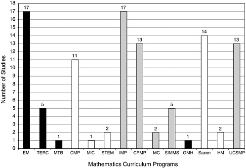
FIGURE 5-1 The distribution of comparative studies across programs. Programs are coded by grade band: black bars = elementary, white bars = middle grades, and gray bars = secondary. In this figure, there are six studies that involved two programs and one study that involved three programs.
NOTE: Five programs (MathScape, MMAP, MMOW/ARISE, Addison-Wesley, and Harcourt) are not shown above since no comparative studies were reviewed.
particular curricular program evaluations, in which case all 19 programs are listed separately. At other times, when we seek to inform ourselves on policy-related issues of funding and evaluating curricular materials, we use the NSF-supported, commercially generated, and UCSMP distinctions. We remind the reader of the artificial aspects of this distinction because at the present time, 18 of the 19 curricula are published commercially. In order to track the question of historical inception and policy implications, a distinction is drawn between the three categories. Figure 5-1 shows the distribution of comparative studies across the 14 programs.
The first result the committee wishes to report is the uneven distribution of studies across the curricula programs. There were 67 coded studies of the NSF curricula, 11 studies of UCSMP, and 17 studies of the commercial publishers. The 14 evaluation studies conducted on the Saxon materials compose the bulk of these 17-non-UCSMP and non-NSF-supported curricular evaluation studies. As these results suggest, we know more about the
evaluations of the NSF-supported curricula and UCSMP than about the evaluations of the commercial programs. We suggest that three factors account for this uneven distribution of studies. First, evaluations have been funded by the NSF both as a part of the original call, and as follow-up to the work in the case of three supplemental awards to two of the curricula programs. Second, most NSF-supported programs and UCSMP were developed at university sites where there is access to the resources of graduate students and research staff. Finally, there was some reported reluctance on the part of commercial companies to release studies that could affect perceptions of competitive advantage. As Figure 5-1 shows, there were quite a few comparative studies of Everyday Mathematics (EM), Connected Mathematics Project (CMP), Contemporary Mathematics in Context (Core-Plus Mathematics Project [CPMP]), Interactive Mathematics Program (IMP), UCSMP, and Saxon.
In the programs with many studies, we note that a significant number of studies were generated by a core set of authors. In some cases, the evaluation reports follow a relatively uniform structure applied to single schools, generating multiple studies or following cohorts over years. Others use a standardized evaluation approach to evaluate sequential courses. Any reports duplicating exactly the same sample, outcome measures, or forms of analysis were eliminated. For example, one study of Mathematics Trailblazers (Carter et al., 2002) reanalyzed the data from the larger ARC Implementation Center study (Sconiers et al., 2002), so it was not included separately. Synthesis studies referencing a variety of evaluation reports are summarized in Chapter 6 , but relevant individual studies that were referenced in them were sought out and included in this comparative review.
Other less formal comparative studies are conducted regularly at the school or district level, but such studies were not included in this review unless we could obtain formal reports of their results, and the studies met the criteria outlined for inclusion in our database. In our conclusions, we address the issue of how to collect such data more systematically at the district or state level in order to subject the data to the standards of scholarly peer review and make it more systematically and fairly a part of the national database on curricular effectiveness.
A standard for evaluation of any social program requires that an impact assessment is warranted only if two conditions are met: (1) the curricular program is clearly specified, and (2) the intervention is well implemented. Absent this assurance, one must have a means of ensuring or measuring treatment integrity in order to make causal inferences. Rossi et al. (1999, p. 238) warned that:
two prerequisites [must exist] for assessing the impact of an intervention. First, the program’s objectives must be sufficiently well articulated to make
it possible to specify credible measures of the expected outcomes, or the evaluator must be able to establish such a set of measurable outcomes. Second, the intervention should be sufficiently well implemented that there is no question that its critical elements have been delivered to appropriate targets. It would be a waste of time, effort, and resources to attempt to estimate the impact of a program that lacks measurable outcomes or that has not been properly implemented. An important implication of this last consideration is that interventions should be evaluated for impact only when they have been in place long enough to have ironed out implementation problems.
These same conditions apply to evaluation of mathematics curricula. The comparative studies in this report varied in the quality of documentation of these two conditions; however, all addressed them to some degree or another. Initially by reviewing the studies, we were able to identify one general design template, which consisted of seven critical decision points and determined that it could be used to develop a framework for conducting our meta-analysis. The seven critical decision points we identified initially were:
Choice of type of design: experimental or quasi-experimental;
For those studies that do not use random assignment: what methods of establishing comparability of groups were built into the design—this includes student characteristics, teacher characteristics, and the extent to which professional development was involved as part of the definition of a curriculum;
Definition of the appropriate unit of analysis (students, classes, teachers, schools, or districts);
Inclusion of an examination of implementation components;
Definition of the outcome measures and disaggregated results by program;
The choice of statistical tests, including statistical significance levels and effect size; and
Recognition of limitations to generalizability resulting from design choices.
These are critical decisions that affect the quality of an evaluation. We further identified a subset of these evaluation studies that met a set of minimum conditions that we termed at least minimally methodologically adequate studies. Such studies are those with the greatest likelihood of shedding light on the effectiveness of these programs. To be classified as at least minimally methodologically adequate, and therefore to be considered for further analysis, each evaluation study was required to:
Include quantifiably measurable outcomes such as test scores, responses to specified cognitive tasks of mathematical reasoning, performance evaluations, grades, and subsequent course taking; and
Provide adequate information to judge the comparability of samples. In addition, a study must have included at least one of the following additional design elements:
A report of implementation fidelity or professional development activity;
Results disaggregated by content strands or by performance by student subgroups; and/or
Multiple outcome measures or precise theoretical analysis of a measured construct, such as number sense, proof, or proportional reasoning.
Using this rubric, the committee identified a subset of 63 comparative studies to classify as at least minimally methodologically adequate and to analyze in depth to inform the conduct of future evaluations. There are those who would argue that any threat to the validity of a study discredits the findings, thus claiming that until we know everything, we know nothing. Others would claim that from the myriad of studies, examining patterns of effects and patterns of variation, one can learn a great deal, perhaps tentatively, about programs and their possible effects. More importantly, we can learn about methodologies and how to concentrate and focus to increase the likelihood of learning more quickly. As Lipsey (1997, p. 22) wrote:
In the long run, our most useful and informative contribution to program managers and policy makers and even to the evaluation profession itself may be the consolidation of our piecemeal knowledge into broader pictures of the program and policy spaces at issue, rather than individual studies of particular programs.
We do not wish to imply that we devalue studies of student affect or conceptions of mathematics, but decided that unless these indicators were connected to direct indicators of student learning, we would eliminate them from further study. As a result of this sorting, we eliminated 19 studies of NSF-supported curricula and 13 studies of commercially generated curricula. Of these, 4 were eliminated for their sole focus on affect or conceptions, 3 were eliminated for their comparative focus on outcomes other than achievement, such as teacher-related variables, and 19 were eliminated for their failure to meet the minimum additional characteristics specified in the criteria above. In addition, six others were excluded from the studies of commercial materials because they were not conducted within the grade-
level band specified by the committee for the selection of that program. From this point onward, all references can be assumed to refer to at least minimally methodologically adequate unless a study is referenced for illustration, in which case we label it with “EX” to indicate that it is excluded in the summary analyses. Studies labeled “EX” are occasionally referenced because they can provide useful information on certain aspects of curricular evaluation, but not on the overall effectiveness.
The at least minimally methodologically adequate studies reported on a variety of grade levels. Figure 5-2 shows the different grade levels of the studies. At times, the choice of grade levels was dictated by the years in which high-stakes tests were given. Most of the studies reported on multiple grade levels, as shown in Figure 5-2 .
Using the seven critical design elements of at least minimally methodologically adequate studies as a design template, we describe the overall database and discuss the array of choices on critical decision points with examples. Following that, we report on the results on the at least minimally methodologically adequate studies by program type. To do so, the results of each study were coded as either statistically significant or not. Those studies
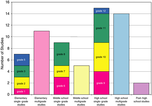
FIGURE 5-2 Single-grade studies by grade and multigrade studies by grade band.
that contained statistically significant results were assigned a percentage of outcomes that are positive (in favor of the treatment curriculum) based on the number of statistically significant comparisons reported relative to the total number of comparisons reported, and a percentage of outcomes that are negative (in favor of the comparative curriculum). The remaining were coded as the percentage of outcomes that are non significant. Then, using seven critical decision points as filters, we identified and examined more closely sets of studies that exhibited the strongest designs, and would therefore be most likely to increase our confidence in the validity of the evaluation. In this last section, we consider alternative hypotheses that could explain the results.
The committee emphasizes that we did not directly evaluate the materials. We present no analysis of results aggregated across studies by naming individual curricular programs because we did not consider the magnitude or rigor of the database for individual programs substantial enough to do so. Nevertheless, there are studies that provide compelling data concerning the effectiveness of the program in a particular context. Furthermore, we do report on individual studies and their results to highlight issues of approach and methodology and to remain within our primary charge, which was to evaluate the evaluations, we do not summarize results of the individual programs.
DESCRIPTION OF COMPARATIVE STUDIES DATABASE ON CRITICAL DECISION POINTS
An experimental or quasi-experimental design.
We separated the studies into experimental and quasiexperimental, and found that 100 percent of the studies were quasiexperimental (Campbell and Stanley, 1966; Cook and Campbell, 1979; and Rossi et al., 1999). 1 Within the quasi-experimental studies, we identified three subcategories of comparative study. In the first case, we identified a study as cross-curricular comparative if it compared the results of curriculum A with curriculum B. A few studies in this category also compared two samples within the curriculum to each other and specified different conditions such as high and low implementation quality.
A second category of a quasi-experimental study involved comparisons that could shed light on effectiveness involving time series studies. These studies compared the performance of a sample of students in a curriculum
|
| One study, by Peters (1992), used random assignment to two classrooms, but was classified as quasi-experimental with its sample size and use of qualitative methods. |
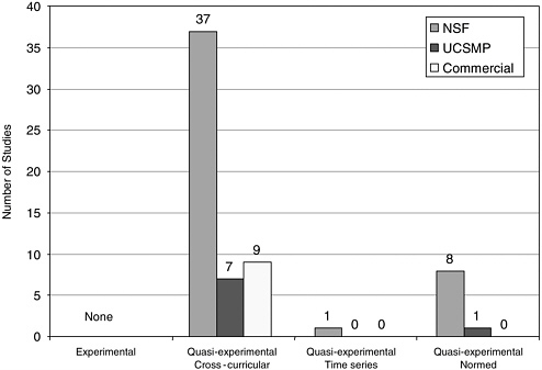
FIGURE 5-3 The number of comparative studies in each category.
under investigation across time, such as in a longitudinal study of the same students over time. A third category of comparative study involved a comparison to some form of externally normed results, such as populations taking state, national, or international tests or prior research assessment from a published study or studies. We categorized these studies and divided them into NSF, UCSMP, and commercial and labeled them by the categories above ( Figure 5-3 ).
In nearly all studies in the comparative group, the titles of experimental curricula were explicitly identified. The only exception to this was the ARC Implementation Center study (Sconiers et al., 2002), where three NSF-supported elementary curricula were examined, but in the results, their effects were pooled. In contrast, in the majority of the cases, the comparison curriculum is referred to simply as “traditional.” In only 22 cases were comparisons made between two identified curricula. Many others surveyed the array of curricula at comparison schools and reported on the most frequently used, but did not identify a single curriculum. This design strategy is used often because other factors were used in selecting comparison groups, and the additional requirement of a single identified curriculum in
these sites would often make it difficult to match. Studies were categorized into specified (including a single or multiple identified curricula) and nonspecified curricula. In the 63 studies, the central group was compared to an NSF-supported curriculum (1), an unnamed traditional curriculum (41), a named traditional curriculum (19), and one of the six commercial curricula (2). To our knowledge, any systematic impact of such a decision on results has not been studied, but we express concern that when a specified curriculum is compared to an unspecified content which is a set of many informal curriculum, the comparison may favor the coherency and consistency of the single curricula, and we consider this possibility subsequently under alternative hypotheses. We believe that a quality study should at least report the array of curricula that comprise the comparative group and include a measure of the frequency of use of each, but a well-defined alternative is more desirable.
If a study was both longitudinal and comparative, then it was coded as comparative. When studies only examined performances of a group over time, such as in some longitudinal studies, it was coded as quasi-experimental normed. In longitudinal studies, the problems created by student mobility were evident. In one study, Carroll (2001), a five-year longitudinal study of Everyday Mathematics, the sample size began with 500 students, 24 classrooms, and 11 schools. By 2nd grade, the longitudinal sample was 343. By 3rd grade, the number of classes increased to 29 while the number of original students decreased to 236 students. At the completion of the study, approximately 170 of the original students were still in the sample. This high rate of attrition from the study suggests that mobility is a major challenge in curricular evaluation, and that the effects of curricular change on mobile students needs to be studied as a potential threat to the validity of the comparison. It is also a challenge in curriculum implementation because students coming into a program do not experience its cumulative, developmental effect.
Longitudinal studies also have unique challenges associated with outcome measures, a study by Romberg et al. (in press) (EX) discussed one approach to this problem. In this study, an external assessment system and a problem-solving assessment system were used. In the External Assessment System, items from the National Assessment of Educational Progress (NAEP) and Third International Mathematics and Science Survey (TIMSS) were balanced across four strands (number, geometry, algebra, probability and statistics), and 20 items of moderate difficulty, called anchor items, were repeated on each grade-specific assessment (p. 8). Because the analyses of the results are currently under way, the evaluators could not provide us with final results of this study, so it is coded as EX.
However, such longitudinal studies can provide substantial evidence of the effects of a curricular program because they may be more sensitive to an
TABLE 5-1 Scores in Percentage Correct by Everyday Mathematics Students and Various Comparison Groups Over a Five-Year Longitudinal Study
|
| Sample Size | 1st Grade | 2nd Grade | 3rd Grade | 4th Grade | 5th Grade |
| EM | n=170-503 | 58 | 62 | 61 | 71 | 75 |
| Traditional U.S. | n=976 | 43 | 53.5 |
|
| 44 |
| Japanese | n=750 | 64 | 71 |
|
| 80 |
| Chinese | n=1,037 | 52 |
|
|
| 76 |
| NAEP Sample | n=18,033 |
|
| 44 | 44 |
|
| NOTE: 1st grade: 44 items; 2nd grade: 24 items; 3rd grade: 22 items; 4th grade: 29 items; and 5th grade: 33 items. SOURCE: Adapted from Carroll (2001). | ||||||
accumulation of modest effects and/or can reveal whether the rates of learning change over time within curricular change.
The longitudinal study by Carroll (2001) showed that the effects of curricula may often accrue over time, but measurements of achievement present challenges to drawing such conclusions as the content and grade level change. A variety of measures were used over time to demonstrate growth in relation to comparison groups. The author chose a set of measures used previously in studies involving two Asian samples and an American sample to provide a contrast to the students in EM over time. For 3rd and 4th grades, where the data from the comparison group were not available, the authors selected items from the NAEP to bridge the gap. Table 5-1 summarizes the scores of the different comparative groups over five years. Scores are reported as the mean percentage correct for a series of tests on number computation, number concepts and applications, geometry, measurement, and data analysis.
It is difficult to compare performances on different tests over different groups over time against a single longitudinal group from EM, and it is not possible to determine whether the students’ performance is increasing or whether the changes in the tests at each grade level are producing the results; thus the results from longitudinal studies lacking a control group or use of sophisticated methodological analysis may be suspect and should be interpreted with caution.
In the Hirsch and Schoen (2002) study, based on a sample of 1,457 students, scores on Ability to Do Quantitative Thinking (ITED-Q) a subset of the Iowa Tests of Education Development, students in Core-Plus showed increasing performance over national norms over the three-year time period. The authors describe the content of the ITED-Q test and point out
that “although very little symbolic algebra is required, the ITED-Q is quite demanding for the full range of high school students” (p. 3). They further point out that “[t]his 3-year pattern is consistent, on average, in rural, urban, and suburban schools, for males and females, for various minority groups, and for students for whom English was not their first language” (p. 4). In this case, one sees that studies over time are important as results over shorter periods may mask cumulative effects of consistent and coherent treatments and such studies could also show increases that do not persist when subject to longer trajectories. One approach to longitudinal studies was used by Webb and Dowling in their studies of the Interactive Mathematics Program (Webb and Dowling, 1995a, 1995b, 1995c). These researchers conducted transcript analyses as a means to examine student persistence and success in subsequent course taking.
The third category of quasi-experimental comparative studies measured student outcomes on a particular curricular program and simply compared them to performance on national tests or international tests. When these tests were of good quality and were representative of a genuine sample of a relevant population, such as NAEP reports or TIMSS results, the reports often provided one a reasonable indicator of the effects of the program if combined with a careful description of the sample. Also, sometimes the national tests or state tests used were norm-referenced tests producing national percentiles or grade-level equivalents. The normed studies were considered of weaker quality in establishing effectiveness, but were still considered valid as examples of comparing samples to populations.
For Studies That Do Not Use Random Assignment: What Methods of Establishing Comparability Across Groups Were Built into the Design
The most fundamental question in an evaluation study is whether the treatment has had an effect on the chosen criterion variable. In our context, the treatment is the curriculum materials, and in some cases, related professional development, and the outcome of interest is academic learning. To establish if there is a treatment effect, one must logically rule out as many other explanations as possible for the differences in the outcome variable. There is a long tradition on how this is best done, and the principle from a design point of view is to assure that there are no differences between the treatment conditions (especially in these evaluations, often there are only the new curriculum materials to be evaluated and a control group) either at the outset of the study or during the conduct of the study.
To ensure the first condition, the ideal procedure is the random assignment of the appropriate units to the treatment conditions. The second condition requires that the treatment is administered reliably during the length of the study, and is assured through the careful observation and
control of the situation. Without randomization, there are a host of possible confounding variables that could differ among the treatment conditions and that are related themselves to the outcome variables. Put another way, the treatment effect is a parameter that the study is set up to estimate. Statistically, an estimate that is unbiased is desired. The goal is that its expected value over repeated samplings is equal to the true value of the parameter. Without randomization at the onset of a study, there is no way to assure this property of unbiasness. The variables that differ across treatment conditions and are related to the outcomes are confounding variables, which bias the estimation process.
Only one study we reviewed, Peters (1992), used randomization in the assignment of students to treatments, but that occurred because the study was limited to one teacher teaching two sections and included substantial qualitative methods, so we coded it as quasi-experimental. Others report partially assigning teachers randomly to treatment conditions (Thompson, et al., 2001; Thompson et al., 2003). Two primary reasons seem to account for a lack of use of pure experimental design. To justify the conduct and expense of a randomized field trial, the program must be described adequately and there must be relative assurance that its implementation has occurred over the duration of the experiment (Peterson et al., 1999). Additionally, one must be sure that the outcome measures are appropriate for the range of performances in the groups and valid relative to the curricula under investigation. Seldom can such conditions be assured for all students and teachers and over the duration of a year or more.
A second reason is that random assignment of classrooms to curricular treatment groups typically is not permitted or encouraged under normal school conditions. As one evaluator wrote, “Building or district administrators typically identified teachers who would be in the study and in only a few cases was random assignment of teachers to UCSMP Algebra or comparison classes possible. School scheduling and teacher preference were more important factors to administrators and at the risk of losing potential sites, we did not insist on randomization” (Mathison et al., 1989, p. 11).
The Joint Committee on Standards for Educational Evaluation (1994, p. 165) committee of evaluations recognized the likelihood of limitations on randomization, writing:
The groups being compared are seldom formed by random assignment. Rather, they tend to be natural groupings that are likely to differ in various ways. Analytical methods may be used to adjust for these initial differences, but these methods are based upon a number of assumptions. As it is often difficult to check such assumptions, it is advisable, when time and resources permit, to use several different methods of analysis to determine whether a replicable pattern of results is obtained.
Does the dearth of pure experimentation render the results of the studies reviewed worthless? Bias is not an “either-or” proposition, but it is a quantity of varying degrees. Through careful measurement of the most salient potential confounding variables, precise theoretical description of constructs, and use of these methods of statistical analysis, it is possible to reduce the amount of bias in the estimated treatment effect. Identification of the most likely confounding variables and their measurement and subsequent adjustments can greatly reduce bias and help estimate an effect that is likely to be more reflective of the true value. The theoretical fully specified model is an alternative to randomization by including relevant variables and thus allowing the unbiased estimation of the parameter. The only problem is realizing when the model is fully specified.
We recognized that we can never have enough knowledge to assure a fully specified model, especially in the complex and unstable conditions of schools. However, a key issue in determining the degree of confidence we have in these evaluations is to examine how they have identified, measured, or controlled for such confounding variables. In the next sections, we report on the methods of the evaluators in identifying and adjusting for such potential confounding variables.
One method to eliminate confounding variables is to examine the extent to which the samples investigated are equated either by sample selection or by methods of statistical adjustments. For individual students, there is a large literature suggesting the importance of social class to achievement. In addition, prior achievement of students must be considered. In the comparative studies, investigators first identified participation of districts, schools, or classes that could provide sufficient duration of use of curricular materials (typically two years or more), availability of target classes, or adequate levels of use of program materials. Establishing comparability was a secondary concern.
These two major factors were generally used in establishing the comparability of the sample:
Student population characteristics, such as demographic characteristics of students in terms of race/ethnicity, economic levels, or location type (urban, suburban, or rural).
Performance-level characteristics such as performance on prior tests, pretest performance, percentage passing standardized tests, or related measures (e.g., problem solving, reading).
In general, four methods of comparing groups were used in the studies we examined, and they permit different degrees of confidence in their results. In the first type, a matching class, school, or district was identified.
Studies were coded as this type if specified characteristics were used to select the schools systematically. In some of these studies, the methodology was relatively complex as correlates of performance on the outcome measures were found empirically and matches were created on that basis (Schneider, 2000; Riordan and Noyce, 2001; and Sconiers et al., 2002). For example, in the Sconiers et al. study, where the total sample of more than 100,000 students was drawn from five states and three elementary curricula are reviewed (Everyday Mathematics, Math Trailblazers [MT], and Investigations [IN], a highly systematic method was developed. After defining eligibility as a “reform school,” evaluators conducted separate regression analyses for the five states at each tested grade level to identify the strongest predictors of average school mathematics score. They reported, “reading score and low-income variables … consistently accounted for the greatest percentage of total variance. These variables were given the greatest weight in the matching process. Other variables—such as percent white, school mobility rate, and percent with limited English proficiency (LEP)—accounted for little of the total variance but were typically significant. These variables were given less weight in the matching process” (Sconiers et al., 2002, p. 10). To further provide a fair and complete comparison, adjustments were made based on regression analysis of the scores to minimize bias prior to calculating the difference in scores and reporting effect sizes. In their results the evaluators report, “The combined state-grade effect sizes for math and total are virtually identical and correspond to a percentile change of about 4 percent favoring the reform students” (p. 12).
A second type of matching procedure was used in the UCSMP evaluations. For example, in an evaluation centered on geometry learning, evaluators advertised in NCTM and UCSMP publications, and set conditions for participation from schools using their program in terms of length of use and grade level. After selecting schools with heterogeneous grouping and no tracking, the researchers used a match-pair design where they selected classes from the same school on the basis of mathematics ability. They used a pretest to determine this, and because the pretest consisted of two parts, they adjusted their significance level using the Bonferroni method. 2 Pairs were discarded if the differences in means and variance were significant for all students or for those students completing all measures, or if class sizes became too variable. In the algebra study, there were 20 pairs as a result of the matching, and because they were comparing three experimental conditions—first edition, second edition, and comparison classes—in the com-
|
| The Bonferroni method is a simple method that allows multiple comparison statements to be made (or confidence intervals to be constructed) while still assuring that an overall confidence coefficient is maintained. |
parison study relevant to this review, their matching procedure identified 8 pairs. When possible, teachers were assigned randomly to treatment conditions. Most results are presented with the eight identified pairs and an accumulated set of means. The outcomes of this particular study are described below in a discussion of outcome measures (Thompson et al., 2003).
A third method was to measure factors such as prior performance or socio-economic status (SES) based on pretesting, and then to use analysis of covariance or multiple regression in the subsequent analysis to factor in the variance associated with these factors. These studies were coded as “control.” A number of studies of the Saxon curricula used this method. For example, Rentschler (1995) conducted a study of Saxon 76 compared to Silver Burdett with 7th graders in West Virginia. He reported that the groups differed significantly in that the control classes had 65 percent of the students on free and reduced-price lunch programs compared to 55 percent in the experimental conditions. He used scores on California Test of Basic Skills mathematics computation and mathematics concepts and applications as his pretest scores and found significant differences in favor of the experimental group. His posttest scores showed the Saxon experimental group outperformed the control group on both computation and concepts and applications. Using analysis of covariance, the computation difference in favor of the experimental group was statistically significant; however, the difference in concepts and applications was adjusted to show no significant difference at the p < .05 level.
A fourth method was noted in studies that used less rigorous methods of selection of sample and comparison of prior achievement or similar demographics. These studies were coded as “compare.” Typically, there was no explicit procedure to decide if the comparison was good enough. In some of the studies, it appeared that the comparison was not used as a means of selection, but rather as a more informal device to convince the reader of the plausibility of the equivalence of the groups. Clearly, the studies that used a more precise method of selection were more likely to produce results on which one’s confidence in the conclusions is greater.
Definition of Unit of Analysis
A major decision in forming an evaluation design is the unit of analysis. The unit of selection or randomization used to assign elements to treatment and control groups is closely linked to the unit of analysis. As noted in the National Research Council (NRC) report (1992, p. 21):
If one carries out the assignment of treatments at the level of schools, then that is the level that can be justified for causal analysis. To analyze the results at the student level is to introduce a new, nonrandomized level into
the study, and it raises the same issues as does the nonrandomized observational study…. The implications … are twofold. First, it is advisable to use randomization at the level at which units are most naturally manipulated. Second, when the unit of observation is at a “lower” level of aggregation than the unit of randomization, then for many purposes the data need to be aggregated in some appropriate fashion to provide a measure that can be analyzed at the level of assignment. Such aggregation may be as simple as a summary statistic or as complex as a context-specific model for association among lower-level observations.
In many studies, inadequate attention was paid to the fact that the unit of selection would later become the unit of analysis. The unit of analysis, for most curriculum evaluators, needs to be at least the classroom, if not the school or even the district. The units must be independently responding units because instruction is a group process. Students are not independent, the classroom—even if the teachers work together in a school on instruction—is not entirely independent, so the school is the unit. Care needed to be taken to ensure that an adequate numbers of units would be available to have sufficient statistical power to detect important differences.
A curriculum is experienced by students in a group, and this implies that individual student responses and what they learn are correlated. As a result, the appropriate unit of assignment and analysis must at least be defined at the classroom or teacher level. Other researchers (Bryk et al., 1993) suggest that the unit might be better selected at an even higher level of aggregation. The school itself provides a culture in which the curriculum is enacted as it is influenced by the policies and assignments of the principal, by the professional interactions and governance exhibited by the teachers as a group, and by the community in which the school resides. This would imply that the school might be the appropriate unit of analysis. Even further, to the extent that such decisions about curriculum are made at the district level and supported through resources and professional development at that level, the appropriate unit could arguably be the district. On a more practical level, we found that arguments can be made for a variety of decisions on the selection of units, and what is most essential is to make a clear argument for one’s choice, to use the same unit in the analysis as in the sample selection process, and to recognize the potential limits to generalization that result from one’s decisions.
We would argue in all cases that reports of how sites are selected must be explicit in the evaluation report. For example, one set of evaluation studies selected sites by advertisements in a journal distributed by the program and in NCTM journals (UCSMP) (Thompson et al., 2001; Thompson et al., 2003). The samples in their studies tended to be affluent suburban populations and predominantly white populations. Other conditions of inclusion, such as frequency of use also might have influenced this outcome,
but it is important that over a set of studies on effectiveness, all populations of students be adequately sampled. When a study is not randomized, adjustments for these confounding variables should be included. In our analysis of equity, we report on the concerns about representativeness of the overall samples and their impact on the generalizability of the results.
Implementation Components
The complexity of doing research on curricular materials introduces a number of possible confounding variables. Due to the documented complexity of curricular implementation, most comparative study evaluators attempt to monitor implementation in some fashion. A valuable outcome of a well-conducted evaluation is to determine not only if the experimental curriculum could ideally have a positive impact on learning, but whether it can survive or thrive in the conditions of schooling that are so variable across sites. It is essential to know what the treatment was, whether it occurred, and if so, to what degree of intensity, fidelity, duration, and quality. In our model in Chapter 3 , these factors were referred to as “implementation components.” Measuring implementation can be costly for large-scale comparative studies; however, many researchers have shown that variation in implementation is a key factor in determining effectiveness. In coding the comparative studies, we identified three types of components that help to document the character of the treatment: implementation fidelity, professional development treatments, and attention to teacher effects.
Implementation Fidelity
Implementation fidelity is a measure of the basic extent of use of the curricular materials. It does not address issues of instructional quality. In some studies, implementation fidelity is synonymous with “opportunity to learn.” In examining implementation fidelity, a variety of data were reported, including, most frequently, the extent of coverage of the curricular material, the consistency of the instructional approach to content in relation to the program’s theory, reports of pedagogical techniques, and the length of use of the curricula at the sample sites. Other less frequently used approaches documented the calendar of curricular coverage, requested teacher feedback by textbook chapter, conducted student surveys, and gauged homework policies, use of technology, and other particular program elements. Interviews with teachers and students, classroom surveys, and observations were the most frequently used data-gathering techniques. Classroom observations were conducted infrequently in these studies, except in cases when comparative studies were combined with case studies, typically with small numbers of schools and classes where observations
were conducted for long or frequent time periods. In our analysis, we coded only the presence or absence of one or more of these methods.
If the extent of implementation was used in interpreting the results, then we classified the study as having adjusted for implementation differences. Across all 63 at least minimally methodologically adequate studies, 44 percent reported some type of implementation fidelity measure, 3 percent reported and adjusted for it in interpreting their outcome measures, and 53 percent recorded no information on this issue. Differences among studies, by study type (NSF, UCSMP, and commercially generated), showed variation on this issue, with 46 percent of NSF reporting or adjusting for implementation, 75 percent of UCSMP, and only 11 percent of the other studies of commercial materials doing so. Of the commercial, non-UCSMP studies included, only one reported on implementation. Possibly, the evaluators for the NSF and UCSMP Secondary programs recognized more clearly that their programs demanded significant changes in practice that could affect their outcomes and could pose challenges to the teachers assigned to them.
A study by Abrams (1989) (EX) 3 on the use of Saxon algebra by ninth graders showed that concerns for implementation fidelity extend to all curricula, even those like Saxon whose methods may seem more likely to be consistent with common practice. Abrams wrote, “It was not the intent of this study to determine the effectiveness of the Saxon text when used as Saxon suggests, but rather to determine the effect of the text as it is being used in the classroom situations. However, one aspect of the research was to identify how the text is being taught, and how closely teachers adhere to its content and the recommended presentation” (p. 7). Her findings showed that for the 9 teachers and 300 students, treatment effects favoring the traditional group (using Dolciani’s Algebra I textbook, Houghton Mifflin, 1980) were found on the algebra test, the algebra knowledge/skills subtest, and the problem-solving test for this population of teachers (fixed effect). No differences were found between the groups on an algebra understanding/applications subtest, overall attitude toward mathematics, mathematical self-confidence, anxiety about mathematics, or enjoyment of mathematics. She suggests that the lack of differences might be due to the ways in which teachers supplement materials, change test conditions, emphasize
|
| Both studies referenced in this section did not meet the criteria for inclusion in the comparative studies, but shed direct light on comparative issues of implementation. The Abrams study was omitted because it examined a program at a grade level outside the specified grade band for that curriculum. Briars and Resnick (2000) did not provide explicit comparison scores to permit one to evaluate the level of student attainment. |
and deemphasize topics, use their own tests, vary the proportion of time spent on development and practice, use calculators and group work, and basically adapt the materials to their own interpretation and method. Many of these practices conflict directly with the recommendations of the authors of the materials.
A study by Briars and Resnick (2000) (EX) in Pittsburgh schools directly confronted issues relevant to professional development and implementation. Evaluators contrasted the performance of students of teachers with high and low implementation quality, and showed the results on two contrasting outcome measures, Iowa Test of Basic Skills (ITBS) and Balanced Assessment. Strong implementers were defined as those who used all of the EM components and provided student-centered instruction by giving students opportunities to explore mathematical ideas, solve problems, and explain their reasoning. Weak implementers were either not using EM or using it so little that the overall instruction in the classrooms was “hardly distinguishable from traditional mathematics instruction” (p. 8). Assignment was based on observations of student behavior in classes, the presence or absence of manipulatives, teacher questionnaires about the programs, and students’ knowledge of classroom routines associated with the program.
From the identification of strong- and weak-implementing teachers, strong- and weak-implementation schools were identified as those with strong- or weak-implementing teachers in 3rd and 4th grades over two consecutive years. The performance of students with 2 years of EM experience in these settings composed the comparative samples. Three pairs of strong- and weak-implementation schools with similar demographics in terms of free and reduced-price lunch (range 76 to 93 percent), student living with only one parent (range 57 to 82 percent), mobility (range 8 to 16 percent), and ethnicity (range 43 to 98 percent African American) were identified. These students’ 1st-grade ITBS scores indicated similarity in prior performance levels. Finally, evaluators predicted that if the effects were due to the curricular implementation and accompanying professional development, the effects on scores should be seen in 1998, after full implementation. Figure 5-4 shows that on the 1998 New Standards exams, placement in strong- and weak-implementation schools strongly affected students’ scores. Over three years, performance in the district on skills, concepts, and problem solving rose, confirming the evaluator’s predictions.
An article by McCaffrey et al. (2001) examining the interactions among instructional practices, curriculum, and student achievement illustrates the point that distinctions are often inadequately linked to measurement tools in their treatment of the terms traditional and reform teaching. In this study, researchers conducted an exploratory factor analysis that led them to create two scales for instructional practice: Reform Practices and Tradi-
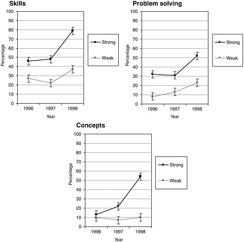
FIGURE 5-4 Percentage of students who met or exceeded the standard. Districtwide grade 4 New Standards Mathematics Reference Examination (NSMRE) performance for 1996, 1997, and 1998 by level of Everyday Mathematics implementation. Percentage of students who achieved the standard. Error bars denote the 99 percent confidence interval for each data point.
SOURCE: Re-created from Briars and Resnick (2000, pp. 19-20).
tional Practices. The reform scale measured the frequency, by means of teacher report, of teacher and student behaviors associated with reform instruction and assessment practices, such as using small-group work, explaining reasoning, representing and using data, writing reflections, or performing tasks in groups. The traditional scale focused on explanations to whole classes, the use of worksheets, practice, and short-answer assessments. There was a –0.32 correlation between scores for integrated curriculum teachers. There was a 0.27 correlation between scores for traditional
curriculum teachers. This shows that it is overly simplistic to think that reform and traditional practices are oppositional. The relationship among a variety of instructional practices is rather more complex as they interact with curriculum and various student populations.
Professional Development
Professional development and teacher effects were separated in our analysis from implementation fidelity. We recognized that professional development could be viewed by the readers of this report in two ways. As indicated in our model, professional development can be considered a program element or component or it can be viewed as part of the implementation process. When viewed as a program element, professional development resources are considered mandatory along with program materials. In relation to evaluation, proponents of considering professional development as a mandatory program element argue that curricular innovations, which involve the introduction of new topics, new types of assessment, or new ways of teaching, must make provision for adequate training, just as with the introduction of any new technology.
For others, the inclusion of professional development in the program elements without a concomitant inclusion of equal amounts of professional development relevant to a comparative treatment interjects a priori disproportionate treatments and biases the results. We hoped for an array of evaluation studies that might shed some empirical light on this dispute, and hence separated professional development from treatment fidelity, coding whether or not studies reported on the amount of professional development provided for the treatment and/or comparison groups. A study was coded as positive if it either reported on the professional development provided on the experimental group or reported the data on both treatments. Across all 63 at least minimally methodologically adequate studies, 27 percent reported some type of professional development measure, 1.5 percent reported and adjusted for it in interpreting their outcome measures, and 71.5 percent recorded no information on the issue.
A study by Collins (2002) (EX) 4 illustrates the critical and controversial role of professional development in evaluation. Collins studied the use of Connected Math over three years, in three middle schools in threat of being classified as low performing in the Massachusetts accountability system. A comparison was made between one school (School A) that engaged
|
| The Collins study lacked a comparison group and is coded as EX. However, it is reported as a case study. |
substantively in professional development opportunities accompanying the program and two that did not (Schools B and C). In the CMP school reports (School A) totals between 100 and 136 hours of professional development were recorded for all seven teachers in grades 6 through 8. In School B, 66 hours were reported for two teachers and in School C, 150 hours were reported for eight teachers over three years. Results showed significant differences in the subsequent performance by students at the school with higher participation in professional development (School A) and it became a districtwide top performer; the other two schools remained at risk for low performance. No controls for teacher effects were possible, but the results do suggest the centrality of professional development for successful implementation or possibly suggest that the results were due to professional development rather than curriculum materials. The fact that these two interpretations cannot be separated is a problem when professional development is given to one and not the other. The effect could be due to textbook or professional development or an interaction between the two. Research designs should be adjusted to consider these issues when different conditions of professional development are provided.
Teacher Effects
These studies make it obvious that there are potential confounding factors of teacher effects. Many evaluation studies devoted inadequate attention to the variable of teacher quality. A few studies (Goodrow, 1998; Riordan and Noyce, 2001; Thompson et al., 2001; and Thompson et al., 2003) reported on teacher characteristics such as certification, length of service, experience with curricula, or degrees completed. Those studies that matched classrooms and reported by matched results rather than aggregated results sought ways to acknowledge the large variations among teacher performance and its impact on student outcomes. We coded any effort to report on possible teacher effects as one indicator of quality. Across all 63 at least minimally methodologically adequate studies, 16 percent reported some type of teacher effect measure, 3 percent reported and adjusted for it in interpreting their outcome measures, and 81 percent recorded no information on this issue.
One can see that the potential confounding factors of teacher effects, in terms of the provision of professional development or the measure of teacher effects, are not adequately considered in most evaluation designs. Some studies mention and give a subjective judgment as to the nature of the problem, but this is descriptive at the most. Hardly any of the studies actually do anything analytical, and because these are such important potential confounding variables, this presents a serious challenge to the efficacy of these studies. Figure 5-5 shows how attention to these factors varies
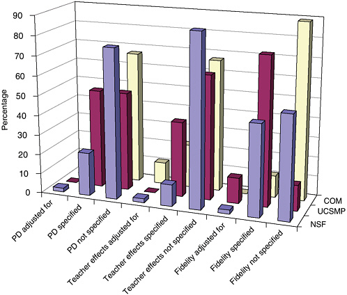
FIGURE 5-5 Treatment of implementation components by program type.
NOTE: PD = professional development.
across program categories among NSF-supported, UCSMP, and studies of commercial materials. In general, evaluations of NSF-supported studies were the most likely to measure these variables; UCSMP had the most standardized use of methods to do so across studies; and commercial material evaluators seldom reported on issues of implementation fidelity.
Identification of a Set of Outcome Measures and Forms of Disaggregation
Using the selected student outcomes identified in the program theory, one must conduct an impact assessment that refers to the design and measurement of student outcomes. In addition to selecting what outcomes should be measured within one’s program theory, one must determine how these outcomes are measured, when those measures are collected, and what
purpose they serve from the perspective of the participants. In the case of curricular evaluation, there are significant issues involved in how these measures are reported. To provide insight into the level of curricular validity, many evaluators prefer to report results by topic, content strand, or item cluster. These reports often present the level of specificity of outcome needed to inform curriculum designers, especially when efforts are made to document patterns of errors, distribution of results across multiple choices, or analyses of student methods. In these cases, whole test scores may mask essential differences in impact among curricula at the level of content topics, reporting only average performance.
On the other hand, many large-scale assessments depend on methods of test equating that rely on whole test scores and make comparative interpretations of different test administrations by content strands of questionable reliability. Furthermore, there are questions such as whether to present only gain scores effect sizes, how to link pretests and posttests, and how to determine the relative curricular sensitivity of various outcome measures.
The findings of comparative studies are reported in terms of the outcome measure(s) collected. To describe the nature of the database with regard to outcome measures and to facilitate our analyses of the studies, we classified each of the included studies on four outcome measure dimensions:
Total score reported;
Disaggregation of content strands, subtest, performance level, SES, or gender;
Outcome measure that was specific to curriculum; and
Use of multiple outcome measures.
Most studies reported a total score, but we did find studies that reported only subtest scores or only scores on an item-by-item basis. For example, in the Ben-Chaim et al. (1998) evaluation study of Connected Math, the authors were interested in students’ proportional reasoning proficiency as a result of use of this curriculum. They asked students from eight seventh-grade classes of CMP and six seventh-grade classes from the control group to solve a variety of tasks categorized as rate and density problems. The authors provide precise descriptions of the cognitive challenges in the items; however, they do not explain if the problems written up were representative of performance on a larger set of items. A special rating form was developed to code responses in three major categories (correct answer, incorrect answer, and no response), with subcategories indicating the quality of the work that accompanied the response. No reports on reliability of coding were given. Performance on standardized tests indicated that control students’ scores were slightly higher than CMP at the beginning of the
year and lower at the end. Twenty-five percent of the experimental group members were interviewed about their approaches to the problems. The CMP students outperformed the control students (53 percent versus 28 percent) overall in providing the correct answers and support work, and 27 percent of the control group gave an incorrect answer or showed incorrect thinking compared to 13 percent of the CMP group. An item-level analysis permitted the researchers to evaluate the actual strategies used by the students. They reported, for example, that 82 percent of CMP students used a “strategy focused on package price, unit price, or a combination of the two; those effective strategies were used by only 56 of 91 control students (62 percent)” (p. 264).
The use of item or content strand-level comparative reports had the advantage that they permitted the evaluators to assess student learning strategies specific to a curriculum’s program theory. For example, at times, evaluators wanted to gauge the effectiveness of using problems different from those on typical standardized tests. In this case, problems were drawn from familiar circumstances but carefully designed to create significant cognitive challenges, and assess how well the informal strategies approach in CMP works in comparison to traditional instruction. The disadvantages of such an approach include the use of only a small number of items and the concerns for reliability in scoring. These studies seem to represent a method of creating hybrid research models that build on the detailed analyses possible using case studies, but still reporting on samples that provide comparative data. It possibly reflects the concerns of some mathematicians and mathematics educators that the effectiveness of materials needs to be evaluated relative to very specific, research-based issues on learning and that these are often inadequately measured by multiple-choice tests. However, a decision not to report total scores led to a trade-off in the reliability and representativeness of the reported data, which must be addressed to increase the objectivity of the reports.
Second, we coded whether outcome data were disaggregated in some way. Disaggregation involved reporting data on dimensions such as content strand, subtest, test item, ethnic group, performance level, SES, and gender. We found disaggregated results particularly helpful in understanding the findings of studies that found main effects, and also in examining patterns across studies. We report the results of the studies’ disaggregation by content strand in our reports of effects. We report the results of the studies’ disaggregation by subgroup in our discussions of generalizability.
Third, we coded whether a study used an outcome measure that the evaluator reported as being sensitive to a particular treatment—this is a subcategory of what was defined in our framework as “curricular validity of measures.” In such studies, the rationale was that readily available measures such as state-mandated tests, norm-referenced standardized tests, and
college entrance examinations do not measure some of the aims of the program under study. A frequently cited instance of this was that “off the shelf” instruments do not measure well students’ ability to apply their mathematical knowledge to problems embedded in complex settings. Thus, some studies constructed a collection of tasks that assessed this ability and collected data on it (Ben-Chaim et al., 1998; Huntley et al., 2000).
Finally, we recorded whether a study used multiple outcome measures. Some studies used a variety of achievement measures and other studies reported on achievement accompanied by measures such as subsequent course taking or various types of affective measures. For example, Carroll (2001, p. 47) reported results on a norm-referenced standardized achievement test as well as a collection of tasks developed in other studies.
A study by Huntley et al. (2000) illustrates how a variety of these techniques were combined in their outcome measures. They developed three assessments. The first emphasized contextualized problem solving based on items from the American Mathematical Association of Two-Year Colleges and others; the second assessment was on context-free symbolic manipulation and a third part requiring collaborative problem solving. To link these measures to the overall evaluation, they articulated an explicit model of cognition based on how one links an applied situation to mathematical activity through processes of formulation and interpretation. Their assessment strategy permitted them to investigate algebraic reasoning as an ability to use algebraic ideas and techniques to (1) mathematize quantitative problem situations, (2) use algebraic principles and procedures to solve equations, and (3) interpret results of reasoning and calculations.
In presenting their data comparing performance on Core-Plus and traditional curriculum, they presented both main effects and comparisons on subscales. Their design of outcome measures permitted them to examine differences in performance with and without context and to conclude with statements such as “This result illustrates that CPMP students perform better than control students when setting up models and solving algebraic problems presented in meaningful contexts while having access to calculators, but CPMP students do not perform as well on formal symbol-manipulation tasks without access to context cues or calculators” (p. 349). The authors go on to present data on the relationship between knowing how to plan or interpret solutions and knowing how to carry them out. The correlations between these variables were weak but significantly different (0.26 for control groups and 0.35 for Core-Plus). The advantage of using multiple measures carefully tied to program theory is that they can permit one to test fine content distinctions that are likely to be the level of adjustments necessary to fine tune and improve curricular programs.
Another interesting approach to the use of outcome measures is found in the UCSMP studies. In many of these studies, evaluators collected infor-
TABLE 5-2 Mean Percentage Correct on the Subject Tests
| Treatment Group | Geometry—Standard | Geometry—UCSMP | Advanced Algebra—UCSMP |
| UCSMP | 43.1, 44.7, 50.5 | 51.2, 54.5 | 56.1, 58.8, 56.1 |
| Comparison | 42.7, 45.5, 51.5 | 36.6, 40.8 | 42.0, 50.1, 50.0 |
| “43.1, 44.7, 50.5” means students were correct on 43.1 percent of the total items, 44.7 percent of the fair items for UCSMP, and 50.5 percent of the items that were taught in both treatments. Too few items to report data. SOURCES: Adapted from Thompson et al. (2001); Thompson et al. (2003). | |||
mation from teachers’ reports and chapter reviews as to whether topics for items on the posttests were taught, calling this an “opportunity to learn” measure. The authors reported results from three types of analyses: (1) total test scores, (2) fair test scores (scores reported by program but only on items on topics taught), and (3) conservative test scores (scores on common items taught in both). Table 5-2 reports on the variations across the multiple- choice test scores for the Geometry study (Thompson et al., 2003) on a standardized test, High School Subject Tests-Geometry Form B , and the UCSMP-constructed Geometry test, and for the Advanced Algebra Study on the UCSMP-constructed Advanced Algebra test (Thompson et al., 2001). The table shows the mean scores for UCSMP classes and comparison classes. In each cell, mean percentage correct is reported first by whole test, then by fair test, and then by conservative test.
The authors explicitly compare the items from the standard Geometry test with the items from the UCSMP test and indicate overlap and difference. They constructed their own test because, in their view, the standard test was not adequately balanced among skills, properties, and real-world uses. The UCSMP test included items on transformations, representations, and applications that were lacking in the national test. Only five items were taught by all teachers; hence in the case of the UCSMP geometry test, there is no report on a conservative test. In the Advanced Algebra evaluation, only a UCSMP-constructed test was viewed as appropriate to cover the treatment of the prior material and alignment to the goals of the new course. These data sets demonstrate the challenge of selecting appropriate outcome measures, the sensitivity of the results to those decisions, and the importance of full disclosure of decision-making processes in order to permit readers to assess the implications of the choices. The methodology utilized sought to ensure that the material in the course was covered adequately by treatment teachers while finding ways to make comparisons that reflected content coverage.
Only one study reported on its outcomes using embedded assessment items employed over the course of the year. In a study of Saxon and UCSMP, Peters (1992) (EX) studied the use of these materials with two classrooms taught by the same teacher. In this small study, he randomly assigned students to treatment groups and then measured their performance on four unit tests composed of items common to both curricula and their progress on the Orleans-Hanna Algebraic Prognosis Test.
Peters’ study showed no significant difference in placement scores between Saxon and UCSMP on the posttest, but did show differences on the embedded assessment. Figure 5-6 (Peters, 1992, p. 75) shows an interesting display of the differences on a “continuum” that shows both the direction and magnitude of the differences and provides a level of concept specificity missing in many reports. This figure and a display ( Figure 5-7 ) in a study by Senk (1991, p. 18) of students’ mean scores on Curriculum A versus Curriculum B with a 10 percent range of differences marked represent two excellent means to communicate the kinds of detailed content outcome information that promises to be informative to curriculum writers, publishers, and school decision makers. In Figure 5-7 , 16 items listed by number were taken from the Second International Mathematics Study. The Functions, Statistics, and Trigonometry sample averaged 41 percent correct on these items whereas the U.S. precalculus sample averaged 38 percent. As shown in the figure, differences of 10 percent or less fall inside the banded area and greater than 10 percent fall outside, producing a display that makes it easy for readers and designers to identify the relative curricular strengths and weaknesses of topics.
While we value detailed outcome measure information, we also recognize the importance of examining curricular impact on students’ standardized test performance. Many developers, but not all, are explicit in rejecting standardized tests as adequate measures of the outcomes of their programs, claiming that these tests focus on skills and manipulations, that they are overly reliant on multiple-choice questions, and that they are often poorly aligned to new content emphases such as probability and statistics, transformations, use of contextual problems and functions, and process skills, such as problem solving, representation, or use of calculators. However, national and state tests are being revised to include more content on these topics and to draw on more advanced reasoning. Furthermore, these high-stakes tests are of major importance in school systems, determining graduation, passing standards, school ratings, and so forth. For this reason, if a curricular program demonstrated positive impact on such measures, we referred to that in Chapter 3 as establishing “curricular alignment with systemic factors.” Adequate performance on these measures is of paramount importance to the survival of reform (to large groups of parents and
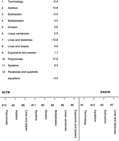
FIGURE 5-6 Continuum of criterion score averages for studied programs.
SOURCE: Peters (1992, p. 75).
school administrators). These examples demonstrate how careful attention to outcomes measures is an essential element of valid evaluation.
In Table 5-3 , we document the number of studies using a variety of types of outcome measures that we used to code the data, and also report on the types of tests used across the studies.
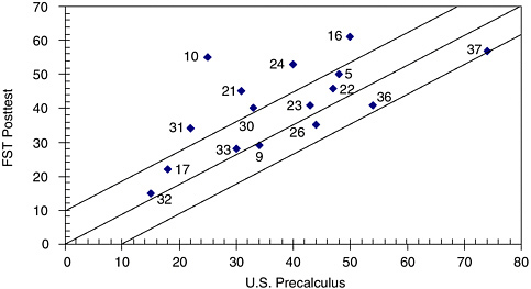
FIGURE 5-7 Achievement (percentage correct) on Second International Mathematics Study (SIMS) items by U.S. precalculus students and functions, statistics, and trigonometry (FST) students.
SOURCE: Re-created from Senk (1991, p. 18).
TABLE 5-3 Number of Studies Using a Variety of Outcome Measures by Program Type
|
| Total Test | Content Strands | Test Match to Program | Multiple Test | ||||
|
| Yes | No | Yes | No | Yes | No | Yes | No |
| NSF | 43 | 3 | 28 | 18 | 26 | 20 | 21 | 25 |
| Commercial | 8 | 1 | 4 | 5 | 2 | 7 | 2 | 7 |
| UCSMP | 7 | 1 | 7 | 1 | 7 | 1 | 7 | 1 |
A Choice of Statistical Tests, Including Statistical Significance and Effect Size
In our first review of the studies, we coded what methods of statistical evaluation were used by different evaluators. Most common were t-tests; less frequently one found Analysis of Variance (ANOVA), Analysis of Co-
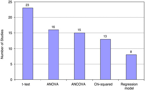
FIGURE 5-8 Statistical tests most frequently used.
variance (ANCOVA), and chi-square tests. In a few cases, results were reported using multiple regression or hierarchical linear modeling. Some used multiple tests; hence the total exceeds 63 ( Figure 5-8 ).
One of the difficult aspects of doing curriculum evaluations concerns using the appropriate unit both in terms of the unit to be randomly assigned in an experimental study and the unit to be used in statistical analysis in either an experimental or quasi-experimental study.
For our purposes, we made the decision that unless the study concerned an intact student population such as the freshman at a single university, where a student comparison was the correct unit, we believed that for statistical tests, the unit should be at least at the classroom level. Judgments were made for each study as to whether the appropriate unit was utilized. This question is an important one because statistical significance is related to sample size, and as a result, studies that inappropriately use the student as the unit of analysis could be concluding significant differences where they are not present. For example, if achievement differences between two curricula are tested in 16 classrooms with 400 students, it will always be easier to show significant differences using scores from those 400 students than using 16 classroom means.
Fifty-seven studies used students as the unit of analysis in at least one test of significance. Three of these were coded as correct because they involved whole populations. In all, 10 studies were coded as using the
TABLE 5-4 Performance on Applied Algebra Problems with Use of Calculators, Part 1
| Treatment | n | M (0-100) | SD |
| Control | 273 | 34.1 | 14.8 |
| CPMP | 320 | 42.6 | 21.3 |
| NOTE: t = -5.69, p < .001. All sites combined SOURCE: Huntley et al. (2000). Reprinted with permission. | |||
TABLE 5-5 Reanalysis of Algebra Performance Data
|
| Site Mean | Independent Samples Dependent | Difference Sample Difference | |
| Site | Control | CPMP | ||
| 1 | 31.7 | 35.5 |
| 3.8 |
| 2 | 26.0 | 49.4 |
| 23.4 |
| 3 | 36.7 | 25.2 |
| -11.5 |
| 4 | 41.9 | 47.7 |
| 5.8 |
| 5 | 29.4 | 38.3 |
| 8.9 |
| 6 | 30.5 | 45.6 |
| 15.1 |
| Average | 32.7 | 40.3 | 7.58 | 7.58 |
| Standard deviation | 5.70 | 9.17 | 7.64 | 11.75 |
| Standard error |
|
| 4.41 | 4.80 |
|
|
| t | 1.7 | 1.6 |
|
|
| p | 0.116 | 0.175 |
|
SOURCE: Huntley et al. (2000). | ||||
correct unit of analysis; hence, 7 studies used teachers or classes, or schools. For some studies where multiple tests were conducted, a judgment was made as to whether the primary conclusions drawn treated the unit of analysis adequately. For example, Huntley et al. (2000) compared the performance of CPMP students with students in a traditional course on a measure of ability to formulate and use algebraic models to answer various questions about relationships among variables. The analysis used students as the unit of analysis and showed a significant difference, as shown in Table 5-4 .
To examine the robustness of this result, we reanalyzed the data using an independent sample t-test and a matched pairs t-test with class means as the unit of analysis in both tests ( Table 5-5 ). As can be seen from the analyses, in neither statistical test was the difference between groups found to be significantly different (p < .05), thus emphasizing the importance of using the correct unit in analyzing the data.
Reanalysis of student-level data using class means will not always result
TABLE 5-6 Mean Percentage Correct on Entire Multiple-Choice Posttest: Second Edition and Non-UCSMP
| School | Pair | UCSMP Second Edition | |||
| Code | ID | n | Mean | SD | OTL |
| J | 18 | 18 | 60.8 | 9.0 | 100 |
| J | 19 | 11 | 58.8 | 13.5 | 100 |
| K | 20 | 22 | 63.8 | 13.0 | 94 |
| K | 21 | 16 | 64.8 | 14.0 | 94 |
| L | 22 | 19 | 57.6 | 16.9 | 92 |
| L | 23 | 13 | 44.7 | 11.2 | 92 |
| M | 24 | 29 | 58.4 | 12.7 | 92 |
| M | 25 | 22 | 39.6 | 13.5 | 92 |
| Overall |
| 150 | 56.1 | 15.4 |
|
| NOTE: The mean is the mean percentage correct on a 36-item multiple-choice posttest. The OTL is the percentage of the items for which teachers reported their students had the opportunity to learn the needed content. Underline indicates statistically significant differences between the mean percentage correct for each pair. | |||||
in a change in finding. Furthermore, using class means as the unit of analysis does not suggest that significant differences will not be found. For example, a study by Thompson et al. (2001) compared the performance of UCSMP students with the performance of students in a more traditional program across several measures of achievement. They found significant differences between UCSMP students and the non-UCSMP students on several measures. Table 5-6 shows results of an analysis of a multiple-choice algebraic posttest using class means as the unit of analysis. Significant differences were found in five of eight separate classroom comparisons, as shown in the table. They also found a significant difference using a matched-pairs t-test on class means.
The lesson to be learned from these reanalyses is that the choice of unit of analysis and the way the data are aggregated can impact study findings in important ways including the extent to which these findings can be generalized. Thus it is imperative that evaluators pay close attention to such considerations as the unit of analysis and the way data are aggregated in the design, implementation, and analysis of their studies.
| Non-UCSMP | |||||||
| n | Mean | SD | OTL | SE | t | df | p |
| 14 | 55.2 | 10.2 | 69 | 3.40 | 1.65 | 30 | 0.110 |
| 15 | 53.7 | 11.0 | 69 | 4.81 | 1.06 | 24 | 0.299 |
| 24 | 45.9 | 10.0 | 72 | 3.41 | 5.22 | 44 |
|
| 23 | 43.0 | 11.9 | 72 | 4.16 | 5.23 | 37 |
|
| 20 | 38.8 | 9.1 | 75 | 4.32 | 4.36 | 37 |
|
| 15 | 38.3 | 11.0 | 75 | 4.20 | 1.52 | 26 | 0.140 |
| 22 | 37.8 | 13.8 | 47 | 3.72 | 5.56 | 49 |
|
| 23 | 30.8 | 9.9 | 47 | 3.52 | 2.51 | 43 |
|
| 156 | 42.0 | 13.1 |
|
|
|
|
|
| A matched-pairs t-test indicates that the differences between the two curricula are significant.
SOURCE: Thompson et al. (2001). Reprinted with permission. | |||||||
Second, effect size has become a relatively common and standard way of gauging the practical significance of the findings. Statistical significance only indicates whether the main-level differences between two curricula are large enough to not be due to chance, assuming they come from the same population. When statistical differences are found, the question remains as to whether such differences are large enough to consider. Because any innovation has its costs, the question becomes one of cost-effectiveness: Are the differences in student achievement large enough to warrant the costs of change? Quantifying the practical effect once statistical significance is established is one way to address this issue. There is a statistical literature for doing this, and for the purposes of this review, the committee simply noted whether these studies have estimated such an effect. However, the committee further noted that in conducting meta-analyses across these studies, effect size was likely to be of little value. These studies used an enormous variety of outcome measures, and even using effect size as a means to standardize units across studies is not sensible when the measures in each
study address such a variety of topics, forms of reasoning, content levels, and assessment strategies.
We note very few studies drew upon the advances in methodologies employed in modeling, which include causal modeling, hierarchical linear modeling (Bryk and Raudenbush, 1992; Bryk et al., 1993), and selection bias modeling (Heckman and Hotz, 1989). Although developing detailed specifications for these approaches is beyond the scope of this review, we wish to emphasize that these methodological advances should be considered within future evaluation designs.
Results and Limitations to Generalizability Resulting from Design Constraints
One also must consider what generalizations can be drawn from the results (Campbell and Stanley, 1966; Caporaso and Roos, 1973; and Boruch, 1997). Generalization is a matter of external validity in that it determines to what populations the study results are likely to apply. In designing an evaluation study, one must carefully consider, in the selection of units of analysis, how various characteristics of those units will affect the generalizability of the study. It is common for evaluators to conflate issues of representativeness for the purpose of generalizability (external validity) and comparativeness (the selection of or adjustment for comparative groups [internal validity]). Not all studies must be representative of the population served by mathematics curricula to be internally valid. But, to be generalizable beyond restricted communities, representativeness must be obtained by the random selection of the basic units. Clearly specifying such limitations to generalizability is critical. Furthermore, on the basis of equity considerations, one must be sure that if overall effectiveness is claimed, that the studies have been conducted and analyzed with reference of all relevant subgroups.
Thus, depending on the design of a study, its results may be limited in generalizability to other populations and circumstances. We identified four typical kinds of limitations on the generalizability of studies and coded them to determine, on the whole, how generalizable the results across studies might be.
First, there were studies whose designs were limited by the ability or performance level of the students in the samples. It was not unusual to find that when new curricula were implemented at the secondary level, schools kept in place systems of tracking that assigned the top students to traditional college-bound curriculum sequences. As a result, studies either used comparative groups who were matched demographically but less skilled than the population as a whole, in relation to prior learning, or their results compared samples of less well-prepared students to samples of students
with stronger preparations. Alternatively, some studies reported on the effects of curricula reform on gifted and talented students or on college-attending students. In these cases, the study results would also limit the generalizability of the results to similar populations. Reports using limited samples of students’ ability and prior performance levels were coded as a limitation to the generalizability of the study.
For example, Wasman (2000) conducted a study of one school (six teachers) and examined the students’ development of algebraic reasoning after one (n=100) and two years (n=73) in CMP. In this school, the top 25 percent of the students are counseled to take a more traditional algebra course, so her experimental sample, which was 61 percent white, 35 percent African American, 3 percent Asian, and 1 percent Hispanic, consisted of the lower 75 percent of the students. She reported on the student performance on the Iowa Algebraic Aptitude Test (IAAT) (1992), in the subcategories of interpreting information, translating symbols, finding relationships, and using symbols. Results for Forms 1 and 2 of the test, for the experimental and norm group, are shown in Table 5-7 for 8th graders.
In our coding of outcomes, this study was coded as showing no significant differences, although arguably its results demonstrate a positive set of
TABLE 5-7 Comparing Iowa Algebraic Aptitude Test (IAAT) Mean Scores of the Connected Mathematics Project Forms 1 and 2 to the Normative Group (8th Graders)
|
| Interpreting Information | Translating Symbols | Finding Relationships | Using Symbols | Total |
| CMP: Form 1 | 9.35 | 8.22 | 9.90 | 8.65 | 36.12 |
| 7th (n=51) | (3.36) | (3.44) | (3.26) | (3.12) | (11.28) |
| CMP: Form 1 | 9.76 | 8.56 | 9.41 | 8.27 | 36.00 |
| 8th (n=41) | (3.89) | (3.64) | (4.13) | (3.74) | (13.65) |
| Norm: Form 1 | 10.03 | 9.55 | 9.14 | 8.87 | 37.59 |
| (n=2,467) | (3.35) | (2.89) | (3.59) | (3.19) | (10.57) |
| CMP: Form 2 | 9.41 | 7.82 | 9.29 | 7.65 | 34.16 |
| 7th (n=49) | (4.05) | (3.03) | (3.57) | (3.35) | (11.47) |
| CMP: Form 2 | 11.28 | 8.66 | 10.94 | 9.81 | 40.69 |
| 8th (n=32) | (3.74) | (3.81) | (3.79) | (3.64) | (12.94) |
| Norm: Form 2 | 10.63 | 8.58 | 8.67 | 9.19 | 37.07 |
| (n=2,467) | (3.78) | (2.91) | (3.84) | (3.17) | (11.05) |
| NOTE: Parentheses indicate standard deviation. SOURCE: Adapted from Wasman (2000). | |||||
outcomes as the treatment group was weaker than the control group. Had the researcher used a prior achievement measure and a different statistical technique, significance might have been demonstrated, although potential teacher effects confound interpretations of results.
A second limitation to generalizability was when comparative studies resided entirely at curriculum pilot site locations, where such sites were developed as a means to conduct formative evaluations of the materials with close contact and advice from teachers. Typically, pilot sites have unusual levels of teacher support, whether it is in the form of daily technical support in the use of materials or technology or increased quantities of professional development. These sites are often selected for study because they have established cooperative agreements with the program developers and other sources of data, such as classroom observations, are already available. We coded whether the study was conducted at a pilot site to signal potential limitations in generalizability of the findings.
Third, studies were also coded as being of limited generalizability if they failed to disaggregate their data by socioeconomic class, race, gender, or some other potentially significant sources of restriction on the claims. We recorded the categories in which disaggregation occurred and compiled their frequency across the studies. Because of the need to open the pipeline to advanced study in mathematics by members of underrepresented groups, we were particularly concerned about gauging the extent to which evaluators factored such variables into their analysis of results and not just in terms of the selection of the sample.
Of the 46 included studies of NSF-supported curricula, 19 disaggregated their data by student subgroup. Nine of 17 studies of commercial materials disaggregated their data. Figure 5-9 shows the number of studies that disaggregated outcomes by race or ethnicity, SES, gender, LEP, special education status, or prior achievement. Studies using multiple categories of disaggregation were counted multiple times by program category.
The last category of restricted generalization occurred in studies of limited sample size. Although such studies may have provided more indepth observations of implementation and reports on professional development factors, the smaller numbers of classrooms and students in the study would limit the extent of generalization that could be drawn from it. Figure 5-10 shows the distribution of sizes of the samples in terms of numbers of students by study type.
Summary of Results by Student Achievement Among Program Types
We present the results of the studies as a means to further investigate their methodological implications. To this end, for each study, we counted across outcome measures the number of findings that were positive, nega-
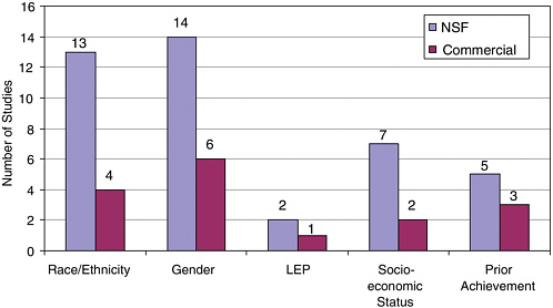
FIGURE 5-9 Disaggregation of subpopulations.
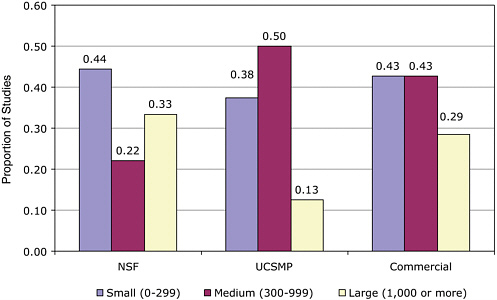
FIGURE 5-10 Proportion of studies by sample size and program.
tive, or indeterminate (no significant difference) and then calculated the proportion of each. We represented the calculation of each study as a triplet (a, b, c) where a indicates the proportion of the results that were positive and statistically significantly stronger than the comparison program, b indicates the proportion that were negative and statistically significantly weaker than the comparison program, and c indicates the proportion that showed no significant difference between the treatment and the comparative group. For studies with a single outcome measure, without disaggregation by content strand, the triplet is always composed of two zeros and a single one. For studies with multiple measures or disaggregation by content strand, the triplet is typically a set of three decimal values that sum to one. For example, a study with one outcome measure in favor of the experimental treatment would be coded (1, 0, 0), while one with multiple measures and mixed results more strongly in favor of the comparative curriculum might be listed as (.20, .50, .30). This triplet would mean that for 20 percent of the comparisons examined, the evaluators reported statistically significant positive results, for 50 percent of the comparisons the results were statistically significant in favor of the comparison group, and for 30 percent of the comparisons no significant difference were found. Overall, the mean score on these distributions was (.54, .07, .40), indicating that across all the studies, 54 percent of the comparisons favored the treatment, 7 percent favored the comparison group, and 40 percent showed no significant difference. Table 5-8 shows the comparison by curricular program types. We present the results by individual program types, because each program type relies on a similar program theory and hence could lead to patterns of results that would be lost in combining the data. If the studies of commercial materials are all grouped together to include UCSMP, their pattern of results is (.38, .11, .51). Again we emphasize that due to our call for increased methodological rigor and the use of multiple methods, this result is not sufficient to establish the curricular effectiveness of these programs as a whole with adequate certainty.
We caution readers that these results are summaries of the results presented across a set of evaluations that meet only the standard of at least
TABLE 5-8 Comparison by Curricular Program Types
| Proportion of Results That Are: | NSF-Supported n=46 | UCSMP n=8 | Commercially Generated n=9 |
| In favor of treatment | .591 | .491 | .285 |
| In favor of comparison | .055 | .087 | .130 |
| Show no significant difference | .354 | .422 | .585 |
minimally methodologically adequate . Calculations of statistical significance of each program’s results were reported by the evaluators; we have made no adjustments for weaknesses in the evaluations such as inappropriate use of units of analysis in calculating statistical significance. Evaluations that consistently used the correct unit of analysis, such as UCSMP, could have fewer reports of significant results as a consequence. Furthermore, these results are not weighted by study size. Within any study, the results pay no attention to comparative effect size or to the established credibility of an outcome measure. Similarly, these results do not take into account differences in the populations sampled, an important consideration in generalizing the results. For example, using the same set of studies as an example, UCSMP studies used volunteer samples who responded to advertisements in their newsletters, resulting in samples with disproportionately Caucasian subjects from wealthier schools compared to national samples. As a result, we would suggest that these results are useful only as baseline data for future evaluation efforts. Our purpose in calculating these results is to permit us to create filters from the critical decision points and test how the results change as one applies more rigorous standards.
Given that none of the studies adequately addressed all of the critical criteria, we do not offer these results as definitive, only suggestive—a hypothesis for further study. In effect, given the limitations of time and support, and the urgency of providing advice related to policy, we offer this filtering approach as an informal meta-analytic technique sufficient to permit us to address our primary task, namely, evaluating the quality of the evaluation studies.
This approach reflects the committee’s view that to deeply understand and improve methodology, it is necessary to scrutinize the results and to determine what inferences they provide about the conduct of future evaluations. Analogous to debates on consequential validity in testing, we argue that to strengthen methodology, one must consider what current methodologies are able (or not able) to produce across an entire series of studies. The remainder of the chapter is focused on considering in detail what claims are made by these studies, and how robust those claims are when subjected to challenge by alternative hypothesis, filtering by tests of increasing rigor, and examining results and patterns across the studies.
Alternative Hypotheses on Effectiveness
In the spirit of scientific rigor, the committee sought to consider rival hypotheses that could explain the data. Given the weaknesses in the designs generally, often these alternative hypotheses cannot be dismissed. However, we believed that only after examining the configuration of results and
alternative hypotheses can the next generation of evaluations be better informed and better designed. We began by generating alternative hypotheses to explain the positive directionality of the results in favor of experimental groups. Alternative hypotheses included the following:
The teachers in the experimental groups tended to be self-selecting early adopters, and thus able to achieve effects not likely in regular populations.
Changes in student outcomes reflect the effects of professional development instruction, or level of classroom support (in pilot sites), and thus inflate the predictions of effectiveness of curricular programs.
Hawthorne effect (Franke and Kaul, 1978) occurs when treatments are compared to everyday practices, due to motivational factors that influence experimental participants.
The consistent difference is due to the coherence and consistency of a single curricular program when compared to multiple programs.
The significance level is only achieved by the use of the wrong unit of analysis to test for significance.
Supplemental materials or new teaching techniques produce the results and not the experimental curricula.
Significant results reflect inadequate outcome measures that focus on a restricted set of activities.
The results are due to evaluator bias because too few evaluators are independent of the program developers.
At the same time, one could argue that the results actually underestimate the performance of these materials and are conservative measures, and their alternative hypotheses also deserve consideration:
Many standardized tests are not sensitive to these curricular approaches, and by eliminating studies focusing on affect, we eliminated a key indicator of the appeal of these curricula to students.
Poor implementation or increased demands on teachers’ knowledge dampens the effects.
Often in the experimental treatment, top-performing students are missing as they are advised to take traditional sequences, rendering the samples unequal.
Materials are not well aligned with universities and colleges because tests for placement and success in early courses focus extensively on algebraic manipulation.
Program implementation has been undercut by negative publicity and the fears of parents concerning change.
There are also a number of possible hypotheses that may be affecting the results in either direction, and we list a few of these:
Examining the role of the teacher in curricular decision making is an important element in effective implementation, and design mandates of evaluation design make this impossible (and the positives and negatives or single- versus dual-track curriculum as in Lundin, 2001).
Local tests that are sensitive to the curricular effects typically are not mandatory and hence may lead to unpredictable performance by students.
Different types and extent of professional development may affect outcomes differentially.
Persistence or attrition may affect the mean scores and are often not considered in the comparative analyses.
One could also generate reasons why the curricular programs produced results showing no significance when one program or the other is actually more effective. This could include high degrees of variability in the results, samples that used the correct unit of analysis but did not obtain consistent participation across enough cases, implementation that did not show enough fidelity to the measures, or outcome measures insensitive to the results. Again, subsequent designs should be better informed by these findings to improve the likelihood that they will produce less ambiguous results and replication of studies could also give more confidence in the findings.
It is beyond the scope of this report to consider each of these alternative hypotheses separately and to seek confirmation or refutation of them. However, in the next section, we describe a set of analyses carried out by the committee that permits us to examine and consider the impact of various critical evaluation design decisions on the patterns of outcomes across sets of studies. A number of analyses shed some light on various alternative hypotheses and may inform the conduct of future evaluations.
Filtering Studies by Critical Decision Points to Increase Rigor
In examining the comparative studies, we identified seven critical decision points that we believed would directly affect the rigor and efficacy of the study design. These decision points were used to create a set of 16 filters. These are listed as the following questions:
Was there a report on comparability relative to SES?
Was there a report on comparability of samples relative to prior knowledge?
Was there a report on treatment fidelity?
Was professional development reported on?
Was the comparative curriculum specified?
Was there any attempt to report on teacher effects?
Was a total test score reported?
Was total test score(s) disaggregated by content strand?
Did the outcome measures match the curriculum?
Were multiple tests used?
Was the appropriate unit of analysis used in their statistical tests?
Did they estimate effect size for the study?
Was the generalizability of their findings limited by use of a restricted range of ability levels?
Was the generalizability of their findings limited by use of pilot sites for their study?
Was the generalizability of their findings limited by not disaggregating their results by subgroup?
Was the generalizability of their findings limited by use of small sample size?
The studies were coded to indicate if they reported having addressed these considerations. In some cases, the decision points were coded dichotomously as present or absent in the studies, and in other cases, the decision points were coded trichotomously, as description presented, absent, or statistically adjusted for in the results. For example, a study may or may not report on the comparability of the samples in terms of race, ethnicity, or socioeconomic status. If a report on SES was given, the study was coded as “present” on this decision; if a report was missing, it was coded as “absent”; and if SES status or ethnicity was used in the analysis to actually adjust outcomes, it was coded as “adjusted for.” For each coding, the table that follows reports the number of studies that met that condition, and then reports on the mean percentage of statistically significant results, and results showing no significant difference for that set of studies. A significance test is run to see if the application of the filter produces changes in the probability that are significantly different. 5
In the cases in which studies are coded into three distinct categories—present, absent, and adjusted for—a second set of filters is applied. First, the studies coded as present or adjusted for are combined and compared to those coded as absent; this is what we refer to as a weak test of the rigor of the study. Second, the studies coded as present or absent are combined and compared to those coded as adjusted for. This is what we refer to as a strong test. For dichotomous codings, there can be as few as three compari-
|
| The significance test used was a chi-square not corrected for discontinuity. |
sons, and for trichotomous codings, there can be nine comparisons with accompanying tests of significance. Trichotomous codes were used for adjustments for SES and prior knowledge, examining treatment fidelity, professional development, teacher effects, and reports on effect sizes. All others were dichotomous.
NSF Studies and the Filters
For example, there were 11 studies of NSF-supported curricula that simply reported on the issues of SES in creating equivalent samples for comparison, and for this subset the mean probabilities of getting positive, negative, or results showing no significant difference were (.47, .10, .43). If no report of SES was supplied (n= 21), those probabilities become (.57, .07, .37), indicating an increase in positive results and a decrease in results showing no significant difference. When an adjustment is made in outcomes based on differences in SES (n=14), the probabilities change to (.72, .00, .28), showing a higher likelihood of positive outcomes. The probabilities that result from filtering should always be compared back to the overall results of (.59, .06, .35) (see Table 5-8 ) so as to permit one to judge the effects of more rigorous methodological constraints. This suggests that a simple report on SES without adjustment is least likely to produce positive outcomes; that is, no report produces the outcomes next most likely to be positive and studies that adjusted for SES tend to have a higher proportion of their comparisons producing positive results.
The second method of applying the filter (the weak test for rigor) for the treatment of the adjustment of SES groups compares the probabilities when a report is either given or adjusted for compared to when no report is offered. The combined percentage of a positive outcome of a study in which SES is reported or adjusted for is (.61, .05, .34), while the percentage for no report remains as reported previously at (.57, .07, .37). A final filter compares the probabilities of the studies in which SES is adjusted for with those that either report it only or do not report it at all. Here we compare the percentage of (.72, .00, .28) to (.53, .08, .37) in what we call a strong test. In each case we compared the probability produced by the whole group to those of the filtered studies and conducted a test of the differences to determine if they were significant. These differences were not significant. These findings indicate that to date, with this set of studies, there is no statistically significant difference in results when one reports or adjusts for changes in SES. It appears that by adjusting for SES, one sees increases in the positive results, and this result deserves a closer examination for its implications should it prove to hold up over larger sets of studies.
We ran tests that report the impact of the filters on the number of studies, the percentage of studies, and the effects described as probabilities
for each of the three study categories, NSF-supported and commercially generated with UCSMP included. We claim that when a pattern of probabilities of results does not change after filtering, one can have more confidence in that pattern. When the pattern of results changes, there is a need for an explanatory hypothesis, and that hypothesis can shed light on experimental design. We propose that this “filtering process” constitutes a test of the robustness of the outcome measures subjected to increasing degrees of rigor by using filtering.
Results of Filtering on Evaluations of NSF-Supported Curricula
For the NSF-supported curricular programs, out of 15 filters, 5 produced a probability that differed significantly at the p<.1 level. The five filters were for treatment fidelity, specification of control group, choosing the appropriate statistical unit, generalizability for ability, and generalizability based on disaggregation by subgroup. For each filter, there were from three to nine comparisons, as we examined how the probabilities of outcomes change as tests were more stringent and across the categories of positive results, negative results, and results with no significant differences. Out of a total of 72 possible tests, only 11 produced a probability that differed significantly at the p < .1 level. With 85 percent of the comparisons showing no significant difference after filtering, we suggest the results of the studies were relatively robust in relation to these tests. At the same time, when rigor is increased for the five filters just listed, the results become generally more ambiguous and signal the need for further research with more careful designs.
Studies of Commercial Materials and the Filters
To ensure enough studies to conduct the analysis (n=17), our filtering analysis of the commercially generated studies included UCSMP (n=8). In this case, there were six filters that produced a probability that differed significantly at the p < .1 level. These were treatment fidelity, disaggregation by content, use of multiple tests, use of effect size, generalizability by ability, and generalizability by sample size. In this case, because there were no studies in some possible categories, there were a total of 57 comparisons, and 9 displayed significant differences in the probabilities after filtering at the p < .1 level. With 84 percent of the comparisons showing no significant difference after filtering, we suggest the results of the studies were relatively robust in relation to these tests. Table 5-9 shows the cases in which significant differences were recorded.
Impact of Treatment Fidelity on Probabilities
A few of these differences are worthy of comment. In the cases of both the NSF-supported and commercially generated curricula evaluation studies, studies that reported treatment fidelity differed significantly from those that did not. In the case of the studies of NSF-supported curricula, it appeared that a report or adjustment on treatment fidelity led to proportions with less positive effects and more results showing no significant differences. We hypothesize that this is partly because larger studies often do not examine actual classroom practices, but can obtain significance more easily due to large sample sizes.
In the studies of commercial materials, the presence or absence of measures of treatment fidelity worked differently. Studies reporting on or adjusting for treatment fidelity tended to have significantly higher probabilities in favor of experimental treatment, less positive effects in fewer of the comparative treatments, and more likelihood of results with no significant differences. We hypothesize, and confirm with a separate analysis, that this is because UCSMP frequently reported on treatment fidelity in their designs while study of Saxon typically did not, and the change represents the preponderance of these different curricular treatments in the studies of commercially generated materials.
Impact of Identification of Curricular Program on Probabilities
The significant differences reported under specificity of curricular comparison also merit discussion for studies of NSF-supported curricula. When the comparison group is not specified, a higher percentage of mean scores in favor of the experimental curricula is reported. In the studies of commercial materials, a failure to name specific curricular comparisons also produced a higher percentage of positive outcomes for the treatment, but the difference was not statistically significant. This suggests the possibility that when a specified curriculum is compared to an unspecified curriculum, reports of impact may be inflated. This finding may suggest that in studies of effectiveness, specifying comparative treatments would provide more rigorous tests of experimental approaches.
When studies of commercial materials disaggregate their results of content strands or use multiple measures, their reports of positive outcomes increase, the negative outcomes decrease, and in one case, the results show no significant differences. Percentage of significant difference was only recorded in one comparison within each one of these filters.
TABLE 5-9 Cases of Significant Differences
| Test | Type of Comparison | Category Code | N= | Probabilities Before Filter | p= |
|
| |||||
| Treatment fidelity | Simple compare | Specified | 21 | .51, .02, .47* | *p =.049 |
|
| Not specified |
| 24 | .68, .09, .23* |
|
|
| Adjusted for |
| 1 | .25, .00, .75 |
|
| Treatment fidelity | Strong test | Adjusted for | 22 | .49*, .02, .49** | *p=.098 |
|
| Reported or not specified |
| 24 | .68*, .09, .23** | **p=.019 |
| Control group specified | Simple compare | Specified | 8 | .33*, .00, .66** | *p=.033 |
|
|
| Not specified | 38 | .65*, .07, .29** | **p=.008 |
| Appropriate unit of analysis | Simple compare | Correct | 5 | .30*, .40**, .30 | *p=.069 |
|
|
| Incorrect | 41 | .63*, .01**, .36 | **p=.000 |
| Generalizability by ability | Simple compare | Limited | 5 | .22*, .41**, .37 | *p=.019 |
|
|
| Not limited | 41 | .64*, .01**, .35 | **p=.000 |
| Generalizability by disaggregated subgroup | Simple compare | Limited | 28 | .48*, .09, .43** | *p=.013 |
|
| Not limited | 18 | .76*, .00, .24** | **p=.085 | |
|
| |||||
| Treatment fidelity | Simple compare | Reported | 7 | .53, .37*, .20 | *p=.032 |
|
|
| Not specified | 9 | .26, .67*, .11 |
|
|
|
| Adjusted for | 1 | .45, .00*, .55 |
|
| Treatment fidelity | Weak test | Adjusted for or | 8 | .52, .33, .25* | *p=.087 |
|
|
| Reported versus | 9 | .26, .67, .11* |
|
|
|
| Not specified |
|
|
|
| Outcomes disaggregated by content strand | Simple compare | Reported | 11 | .50, .37, .22* | *p=.052 |
|
| Not reported | 6 | .17, .77, .10* |
| |
| Outcomes using multiple tests | Simple compare | Yes | 9 | .55*, .35, .19 | *p=.076 |
|
|
| No | 8 | .20*, .68, .20 |
|
| Effect size reported | Simple compare | Yes | 3 | .72, .05, .29* | *p=.029 |
|
|
| No | 14 | .31, .61, .16* |
|
| Generalization by ability | Simple compare | Limited | 4 | .23, .41*, .32 | *p=.004 |
|
|
| Not limited | 14 | .42, .53, .09 |
|
| Generalization by sample size | Simple compare | Limited | 6 | .57, .23, .27* | *p=.036 |
|
|
| Not limited | 11 | .28, .66, .10* |
|
| NOTE: In the comparisons shown, only the comparisons marked by an asterisk showed significant differences at p<.1. Probabilitie s are estimated for each significant difference. | |||||
Impact of Units of Analysis on Probabilities 6
For the evaluations of the NSF-supported materials, a significant difference was reported on the outcomes for the studies that used the correct unit of analysis compared to those that did not. The percentage for those with the correct unit were (.30, .40, .30) compared to (.63, .01, .36) for those that used the incorrect result. These results suggest that our prediction that using the correct unit of analysis would decrease the percentage of positive outcomes is likely to be correct. It also suggests that the most serious threat to the apparent conclusions of these studies comes from selecting an incorrect unit of analysis. It causes a decrease in favorable results, making the results more ambiguous, but never reverses the direction of the effect. This is a concern that merits major attention in the conduct of further studies.
For the commercially generated studies, most of the ones coded with the correct unit of analysis were UCSMP studies. Because of the small number of studies involved, we could not break out from the overall filtering of studies of commercial materials, but report this issue to assist readers in interpreting the relative patterns of results.
Impact of Generalizability on Probabilities
Both types of studies yielded significant differences for some of the comparisons coded as restrictions to generalizability. Investigating these is important in order to understand the effects of these curricular programs on different subpopulations of students. In the case of the studies of commercially generated materials, significantly different results occurred in the categories of ability and sample size. In the studies of NSF-supported materials, the significant differences occurred in ability and disaggregation by subgroups.
In relation to generalizability, the studies of NSF-supported curricula reported significantly more positive results in favor of the treatment when they included all students. Because studies coded as “limited by ability” were restricted either by focusing only on higher achieving students or on lower achieving students, we sorted these two groups. For higher performing students (n=3), the probabilities of effects were (.11, .67, .22). For lower
|
| It should be noted that of the five studies in which the correct unit of analysis was used, two of these were population studies of freshmen entering college, and these reported few results in favor of the experimental treatments. However, the high proportion of these studies involving college students may skew this particular result relative to the preponderance of other studies involving K-12 students. |
performing students (n=2), the probabilities were (.39, .025, .59). The first two comparisons are significantly different at p < .05. These findings are based on only a total of five studies, but they suggest that these programs may be serving the weaker ability students more effectively than the stronger ability students, serving both less well than they serve whole heterogeneous groups. For the studies of commercial materials, there were only three studies that were restricted to limited populations. The results for those three studies were (.23, .41, .32) and for all students (n=14) were (.42, .53, .09). These studies were significantly different at p = .004. All three studies included UCSMP and one also included Saxon and was limited by serving primarily high-performing students. This means both categories of programs are showing weaker results when used with high-ability students.
Finally, the studies on NSF-supported materials were disaggregated by subgroups for 28 studies. A complete analysis of this set follows, but the studies that did not report results disaggregated by subgroup generated probabilities of results of (.48, .09, .43) whereas those that did disaggregate their results reported (.76, 0, .24). These gains in positive effects came from significant losses in reporting no significant differences. Studies of commercial materials also reported a small decrease in likelihood of negative effects for the comparison program when disaggregation by subgroup is reported offset by increases in positive results and results with no significant differences, although these comparisons were not significantly different. A further analysis of this topic follows.
Overall, these results suggest that increased rigor seems to lead in general to less strong outcomes, but never reports of completely contrary results. These results also suggest that in recommending design considerations to evaluators, there should be careful attention to having evaluators include measures of treatment fidelity, considering the impact on all students as well as one particular subgroup; using the correct unit of analysis; and using multiple tests that are also disaggregated by content strand.
Further Analyses
We conducted four further analyses: (1) an analysis of the outcome probabilities by test type; (2) content strands analysis; (3) equity analysis; and (4) an analysis of the interactions of content and equity by grade band. Careful attention to the issues of content strand, equity, and interaction is essential for the advancement of curricular evaluation. Content strand analysis provides the detail that is often lost by reporting overall scores; equity analysis can provide essential information on what subgroups are adequately served by the innovations, and analysis by content and grade level can shed light on the controversies that evolve over time.
Analysis by Test Type
Different studies used varied combinations of outcome measures. Because of the importance of outcome measures on test results, we chose to examine whether the probabilities for the studies changed significantly across different types of outcome measures (national test, local test). The most frequent use of tests across all studies was a combination of national and local tests (n=18 studies), a local test (n=16), and national tests (n=17). Other uses of test combinations were used by three studies or less. The percentages of various outcomes by test type in comparison to all studies are described in Table 5-10 .
These data ( Table 5-11 ) suggest that national tests tend to produce less positive results, and with the resulting gains falling into results showing no significant differences, suggesting that national tests demonstrate less curricular sensitivity and specificity.
TABLE 5-10 Percentage of Outcomes by Test Type
| Test Type | National/Local | Local Only | National Only | All Studies |
| All studies | (.48, .18, .34) n=18 | (.63, .03, .34) n=16 | (.31, .05, .64) n= 3 | (.54, .07, .40) n=63 |
| NOTE: The first set of numbers in the parenthesis represent the percentage of outcomes that are positive, the second set of numbers in the parenthesis represent the percentage of outcomes that are negative, and the third set of numbers represent the percentage of outcomes that are nonsignificant. | ||||
TABLE 5-11 Percentage of Outcomes by Test Type and Program Type
| Test Type | National/Local | Local Only | National Only | All Studies |
| NSF effects | (.52, .15, .34) n=14 | (.57, .03, .39) n=14 | (.44, .00, .56) n=4 | (.59, .06, .35) n=46 |
| UCSMP effects | (.41, .18, .41) n=3 | *** | *** | (.49, .09, .42) n=8 |
| Commercial effects | ** | ** | (.29, .08, .63) n=8 | (.29, .13, .59) n=9 |
| NOTE: The first set of numbers in the parenthesis represent the percentage of outcomes that are positive, the second set of numbers represent the percentage of outcomes that are negative, and the third set of numbers represent the percentage of outcomes that are nonsignificant. | ||||
TABLE 5-12 Number of Studies That Disaggregated by Content Strand
| Program Type | Elementary | Middle | High School | Total |
| NSF-supported | 14 | 6 | 9 | 29 |
| Commercially generated | 0 | 4 | 5 | 9 |
Content Strand
Curricular effectiveness is not an all-or-nothing proposition. A curriculum may be effective in some topics and less effective in others. For this reason, it is useful for evaluators to include an analysis of curricular strands and to report on the performance of students on those strands. To examine this issue, we conducted an analysis of the studies that reported their results by content strand. Thirty-eight studies did this; the breakdown is shown in Table 5-12 by type of curricular program and grade band.
To examine the evaluations of these content strands, we began by listing all of the content strands reported across studies as well as the frequency of report by the number of studies at each grade band. These results are shown in Figure 5-11 , which is broken down by content strand, grade level, and program type.
Although there are numerous content strands, some of them were reported on infrequently. To allow the analysis to focus on the key results from these studies, we separated out the most frequently reported on strands, which we call the “major content strands.” We defined these as strands that were examined in at least 10 percent of the studies. The major content strands are marked with an asterisk in the Figure 5-11 . When we conduct analyses across curricular program types or grade levels, we use these to facilitate comparisons.
A second phase of our analysis was to examine the performance of students by content strand in the treatment group in comparison to the control groups. Our analysis was conducted across the major content strands at the level of NSF-supported versus commercially generated, initially by all studies and then by grade band. It appeared that such analysis permitted some patterns to emerge that might prove helpful to future evaluators in considering the overall effectiveness of each approach. To do this, we then coded the number of times any particular strand was measured across all studies that disaggregated by content strand. Then, we coded the proportion of times that this strand was reported as favoring the experimental treatment, favoring the comparative curricula, or showing no significant difference. These data are presented across the major content strands for the NSF-supported curricula ( Figure 5-12 ) and the commercially generated curricula, ( Figure 5-13 ) (except in the case of the elemen-
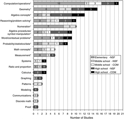
FIGURE 5-11 Study counts for all content strands.
tary curricula where no data were available) in the forms of percentages, with the frequencies listed in the bars.
The presentation of results by strands must be accompanied by the same restrictions as stated previously. These results are based on studies identified as at least minimally methodologically adequate. The quality of the outcome measures in measuring the content strands has not been examined. Their results are coded in relation to the comparison group in the study and are indicated as statistically in favor of the program, as in favor of the comparative program, or as showing no significant differences. The results are combined across studies with no weighting by study size. Their results should be viewed as a means for the identification of topics for potential future study. It is completely possible that a refinement of methodologies may affect the future patterns of results, so the results are to be viewed as tentative and suggestive.
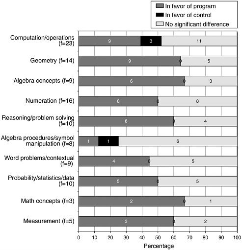
FIGURE 5-12 Major content strand result: All NSF (n=27).
According to these tentative results, future evaluations should examine whether the NSF-supported programs produce sufficient competency among students in the areas of algebraic manipulation and computation. In computation, approximately 40 percent of the results were in favor of the treatment group, no significant differences were reported in approximately 50 percent of the results, and results in favor of the comparison were revealed 10 percent of the time. Interpreting that final proportion of no significant difference is essential. Some would argue that because computation has not been emphasized, findings of no significant differences are acceptable. Others would suggest that such findings indicate weakness, because the development of the materials and accompanying professional development yielded no significant difference in key areas.
FIGURE 5-13 Major content strand result: All commercial (n=8).
From Figure 5-13 of findings from studies of commercially generated curricula, it appears that mixed results are commonly reported. Thus, in evaluations of commercial materials, lack of significant differences in computations/operations, word problems, and probability and statistics suggest that careful attention should be given to measuring these outcomes in future evaluations.
Overall, the grade band results for the NSF-supported programs—while consistent with the aggregated results—provide more detail. At the elementary level, evaluations of NSF-supported curricula (n=12) report better performance in mathematics concepts, geometry, and reasoning and problem solving, and some weaknesses in computation. No content strand analysis for commercially generated materials was possible. Evaluations
(n=6) at middle grades of NSF-supported curricula showed strength in measurement, geometry, and probability and statistics and some weaknesses in computation. In the studies of commercial materials, evaluations (n=4) reported favorable results in reasoning and problem solving and some unfavorable results in algebraic procedures, contextual problems, and mathematics concepts. Finally, at the high school level, the evaluations (n=9) by content strand for the NSF-supported curricula showed strong favorable results in algebra concepts, reasoning/problem solving, word problems, probability and statistics, and measurement. Results in favor of the control were reported in 25 percent of the algebra procedures and 33 percent of computation measures.
For the studies of commercial materials (n=4), only the geometry results favor the control group 25 percent of the time, with 50 percent having favorable results. Algebra concepts, reasoning, and probability and statistics also produced favorable results.
Equity Analysis of Comparative Studies
When the goal of providing a standards-based curriculum to all students was proposed, most people could recognize its merits: the replacement of dull, repetitive, largely dead-end courses with courses that would lead all students to be able, if desired and earned, to pursue careers in mathematics-reliant fields. It was clear that the NSF-supported projects, a stated goal of which was to provide standards-based courses to all students, called for curricula that would address the problem of too few students persisting in the study of mathematics. For example, as stated in the NSF Request for Proposals (RFP):
Rather than prematurely tracking students by curricular objectives, secondary school mathematics should provide for all students a common core of mainstream mathematics differentiated instructionally by level of abstraction and formalism, depth of treatment and pace (National Science Foundation, 1991, p. 1). In the elementary level solicitation, a similar statement on causes for all students was made (National Science Foundation, 1988, pp. 4-5).
Some, but not enough attention has been paid to the education of students who fall below the average of the class. On the other hand, because the above average students sometimes do not receive a demanding education, it may be incorrectly assumed they are easy to teach (National Science Foundation, 1989, p. 2).
Likewise, with increasing numbers of students in urban schools, and increased demographic diversity, the challenges of equity are equally significant for commercial publishers, who feel increasing pressures to demonstrate the effectiveness of their products in various contexts.
The problem was clearly identified: poorer performance by certain subgroups of students (minorities—non-Asian, LEP students, sometimes females) and a resulting lack of representation of such groups in mathematics-reliant fields. In addition, a secondary problem was acknowledged: Highly talented American students were not being provided adequate challenge and stimulation in comparison with their international counterparts. We relied on the concept of equity in examining the evaluation. Equity was contrasted to equality, where one assumed all students should be treated exactly the same (Secada et al., 1995). Equity was defined as providing opportunities and eliminating barriers so that the membership in a subgroup does not subject one to undue and systematically diminished possibility of success in pursuing mathematical study. Appropriate treatment therefore varies according to the needs of and obstacles facing any subgroup.
Applying the principles of equity to evaluate the progress of curricular programs is a conceptually thorny challenge. What is challenging is how to evaluate curricular programs on their progress toward equity in meeting the needs of a diverse student body. Consider how the following questions provide one with a variety of perspectives on the effectiveness of curricular reform regarding equity:
Does one expect all students to improve performance, thus raising the bar, but possibly not to decrease the gap between traditionally well-served and under-served students?
Does one focus on reducing the gap and devote less attention to overall gains, thus closing the gap but possibly not raising the bar?
Or, does one seek evidence that progress is made on both challenges—seeking progress for all students and arguably faster progress for those most at risk?
Evaluating each of the first two questions independently seems relatively straightforward. When one opts for a combination of these two, the potential for tensions between the two becomes more evident. For example, how can one differentiate between the case in which the gap is closed because talented students are being underchallenged from the case in which the gap is closed because the low-performing students improved their progress at an increased rate? Many believe that nearly all mathematics curricula in this country are insufficiently challenging and rigorous. Therefore achieving modest gains across all ability levels with evidence of accelerated progress by at-risk students may still be criticized for failure to stimulate the top performing student group adequately. Evaluating curricula with regard to this aspect therefore requires judgment and careful methodological attention.
Depending on one’s view of equity, different implications for the collection of data follow. These considerations made examination of the quality of the evaluations as they treated questions of equity challenging for the committee members. Hence we spell out our assumptions as precisely as possible:
Evaluation studies should include representative samples of student demographics, which may require particular attention to the inclusion of underrepresented minority students from lower socioeconomic groups, females, and special needs populations (LEP, learning disabled, gifted and talented students) in the samples. This may require one to solicit participation by particular schools or districts, rather than to follow the patterns of commercial implementation, which may lead to an unrepresentative sample in aggregate.
Analysis of results should always consider the impact of the program on the entire spectrum of the sample to determine whether the overall gains are distributed fairly among differing student groups, and not achieved as improvements in the mean(s) of an identifiable subpopulation(s) alone.
Analysis should examine whether any group of students is systematically less well served by curricular implementation, causing losses or weakening the rate of gains. For example, this could occur if one neglected the continued development of programs for gifted and talented students in mathematics in order to implement programs focused on improving access for underserved youth, or if one improved programs solely for one group of language learners, ignoring the needs of others, or if one’s study systematically failed to report high attrition affecting rates of participation of success or failure.
Analyses should examine whether gaps in scores between significantly disadvantaged or underperforming subgroups and advantaged subgroups are decreasing both in relation to eliminating the development of gaps in the first place and in relation to accelerating improvement for underserved youth relative to their advantaged peers at the upper grades.
In reviewing the outcomes of the studies, the committee reports first on what kinds of attention to these issues were apparent in the database, and second on what kinds of results were produced. Some of the studies used multiple methods to provide readers with information on these issues. In our report on the evaluations, we both provide descriptive information on the approaches used and summarize the results of those studies. Developing more effective methods to monitor the achievement of these objectives may need to go beyond what is reported in this study.
Among the 63 at least minimally methodologically adequate studies, 26 reported on the effects of their programs on subgroups of students. The
TABLE 5-13 Most Common Subgroups Used in the Analyses and the Number of Studies That Reported on That Variable
| Identified Subgroup | Number of Studies of NSF-Supported | Number of Studies of Commercially Generated | Total |
| Gender | 14 | 5 | 19 |
| Race and ethnicity | 14 | 2 | 16 |
| Socioeconomic status | 8 | 2 | 10 |
| Achievement levels | 5 | 3 | 8 |
| English as a second language (ESL) | 2 | 1 | 3 |
| Total | 43 | 13 | 56 |
| Achievement levels: Outcome data are reported in relation to categorizations by quartiles or by achievement level based on independent test. | |||
other 37 reported on the effects of the curricular intervention on means of whole groups and their standard deviations, but did not report on their data in terms of the impact on subpopulations. Of those 26 evaluations, 19 studies were on NSF-supported programs and 7 were on commercially generated materials. Table 5-13 reports the most common subgroups used in the analyses and the number of studies that reported on that variable. Because many studies used multiple categories for disaggregation (ethnicity, SES, and gender), the number of reports is more than double the number of studies. For this reason, we report the study results in terms of the “frequency of reports on a particular subgroup” and distinguish this from what we refer to as “study counts.” The advantage of this approach is that it permits reporting on studies that investigated multiple ways to disaggregate their data. The disadvantage is that in a sense, studies undertaking multiple disaggregations become overrepresented in the data set as a result. A similar distinction and approach were used in our treatment of disaggregation by content strands.
It is apparent from these data that the evaluators of NSF-supported curricula documented more equity-based outcomes, as they reported 43 of the 56 comparisons. However, the same percentage of the NSF-supported evaluations disaggregated their results by subgroup, as did commercially generated evaluations (41 percent in both cases). This is an area where evaluations of curricula could benefit greatly from standardization of ex-
pectation and methodology. Given the importance of the topic of equity, it should be standard practice to include such analyses in evaluation studies.
In summarizing these 26 studies, the first consideration was whether representative samples of students were evaluated. As we have learned from medical studies, if conclusions on effectiveness are drawn without careful attention to representativeness of the sample relative to the whole population, then the generalizations drawn from the results can be seriously flawed. In Chapter 2 we reported that across the studies, approximately 81 percent of the comparative studies and 73 percent of the case studies reported data on school location (urban, suburban, rural, or state/region), with suburban students being the largest percentage in both study types. The proportions of students studied indicated a tendency to undersample urban and rural populations and oversample suburban schools. With a high concentration of minorities and lower SES students in these areas, there are some concerns about the representativeness of the work.
A second consideration was to see whether the achievement effects of curricular interventions were achieved evenly among the various subgroups. Studies answered this question in different ways. Most commonly, evaluators reported on the performance of various subgroups in the treatment conditions as compared to those same subgroups in the comparative condition. They reported outcome scores or gains from pretest to posttest. We refer to these as “between” comparisons.
Other studies reported on the differences among subgroups within an experimental treatment, describing how well one group does in comparison with another group. Again, these reports were done in relation either to outcome measures or to gains from pretest to posttest. Often these reports contained a time element, reporting on how the internal achievement patterns changed over time as a curricular program was used. We refer to these as “within” comparisons.
Some studies reported both between and within comparisons. Others did not report findings by comparing mean scores or gains, but rather created regression equations that predicted the outcomes and examined whether demographic characteristics are related to performance. Six studies (all on NSF-supported curricula) used this approach with variables related to subpopulations. Twelve studies used ANCOVA or Multiple Analysis of Variance (MANOVA) to study disaggregation by subgroup, and two reported on comparative effect sizes. In the studies using statistical tests other than t-tests or Chi-squares, two were evaluations of commercially generated materials and the rest were of NSF-supported materials.
Of the studies that reported on gender (n=19), the NSF-supported ones (n=13) reported five cases in which the females outperformed their counterparts in the controls and one case in which the female-male gap decreased within the experimental treatments across grades. In most cases, the studies
present a mixed picture with some bright spots, with the majority showing no significant difference. One study reported significant improvements for African-American females.
In relation to race, 15 of 16 reports on African Americans showed positive effects in favor of the treatment group for NSF-supported curricula. Two studies reported decreases in the gaps between African Americans and whites or Asians. One of the two evaluations of African Americans, performance reported for the commercially generated materials, showed significant positive results, as mentioned previously.
For Hispanic students, 12 of 15 reports of the NSF-supported materials were significantly positive, with the other 3 showing no significant difference. One study reported a decrease in the gaps in favor of the experimental group. No evaluations of commercially generated materials were reported on Hispanic populations. Other reports on ethnic groups occurred too seldom to generalize.
Students from lower socioeconomic groups fared well, according to reported evaluations of NSF-supported materials (n=8), in that experimental groups outperformed control groups in all but one case. The one study of commercially generated materials that included SES as a variable reported no significant difference. For students with limited English proficiency, of the two evaluations of NSF-supported materials, one reported significantly more positive results for the experimental treatment. Likewise, one study of commercially generated materials yielded a positive result at the elementary level.
We also examined the data for ability differences and found reports by quartiles for a few evaluation studies. In these cases, the evaluations showed results across quartiles in favor of the NSF-supported materials. In one case using the same program, the lower quartiles showed the most improvement, and in the other, the gains were in the middle and upper groups for the Iowa Test of Basic Skills and evenly distributed for the informal assessment.
Summary Statements
After reviewing these studies, the committee observed that examining differences by gender, race, SES, and performance levels should be examined as a regular part of any review of effectiveness. We would recommend that all comparative studies report on both “between” and “within” comparisons so that the audience of an evaluation can simply and easily consider the level of improvement, its distribution across subgroups, and the impact of curricular implementation on any gaps in performance. Each of the major categories—gender, race/ethnicity, SES, and achievement level—contributes a significant and contrasting view of curricular impact. Further-
more, more sophisticated accounts would begin to permit, across studies, finer distinctions to emerge, such as the effect of a program on young African-American women or on first generation Asian students.
In addition, the committee encourages further study and deliberation on the use of more complex approaches to the examination of equity issues. This is particularly important due to the overlaps among these categories, where poverty can show itself as its own variable but also may be highly correlated to prior performance. Hence, the use of one variable can mask differences that should be more directly attributable to another. The committee recommends that a group of measurement and equity specialists confer on the most effective design to advance on these questions.
Finally, it is imperative that evaluation studies systematically include demographically representative student populations and distinguish evaluations that follow the commercial patterns of use from those that seek to establish effectiveness with a diverse student population. Along these lines, it is also important that studies report on the impact data on all substantial ethnic groups, including whites. Many studies, perhaps because whites were the majority population, failed to report on this ethnic group in their analyses. As we saw in one study, where Asian students were from poor homes and first generation, any subgroup can be an at-risk population in some setting, and because gains in means may not necessarily be assumed to translate to gains for all subgroups or necessarily for the majority subgroup. More complete and thorough descriptions and configurations of characteristics of the subgroups being served at any location—with careful attention to interactions—is needed in evaluations.
Interactions Among Content and Equity, by Grade Band
By examining disaggregation by content strand by grade levels, along with disaggregation by diverse subpopulations, the committee began to discover grade band patterns of performance that should be useful in the conduct of future evaluations. Examining each of these issues in isolation can mask some of the overall effects of curricular use. Two examples of such analysis are provided. The first example examines all the evaluations of NSF-supported curricula from the elementary level. The second examines the set of evaluations of NSF-supported curricula at the high school level, and cannot be carried out on evaluations of commercially generated programs because they lack disaggregation by student subgroup.
Example One
At the elementary level, the findings of the review of evaluations of data on effectiveness of NSF-supported curricula report consistent patterns of
benefits to students. Across the studies, it appears that positive results are enhanced when accompanied by adequate professional development and the use of pedagogical methods consistent with those indicated by the curricula. The benefits are most consistently evidenced in the broadening topics of geometry, measurement, probability, and statistics, and in applied problem solving and reasoning. It is important to consider whether the outcome measures in these areas demonstrate a depth of understanding. In early understanding of fractions and algebra, there is some evidence of improvement. Weaknesses are sometimes reported in the areas of computational skills, especially in the routinization of multiplication and division. These assertions are tentative due to the possible flaws in designs but quite consistent across studies, and future evaluations should seek to replicate, modify, or discredit these results.
The way to most efficiently and effectively link informal reasoning and formal algorithms and procedures is an open question. Further research is needed to determine how to most effectively link the gains and flexibility associated with student-generated reasoning to the automaticity and generalizability often associated with mastery of standard algorithms.
The data from these evaluations at the elementary level generally present credible evidence of increased success in engaging minority students and students in poverty based on reported gains that are modestly higher for these students than for the comparative groups. What is less well documented in the studies is the extent to which the curricula counteract the tendencies to see gaps emerge and result in long-term persistence in performance by gender and minority group membership as they move up the grades. However, the evaluations do indicate that these curricula can help, and almost never do harm. Finally, on the question of adequate challenge for advanced and talented students, the data are equivocal. More attention to this issue is needed.
Example Two
The data at the high school level produced the most conflicting results, and in conducting future evaluations, evaluators will need to examine this level more closely. We identify the high school as the crucible for curricular change for three reasons: (1) the transition to postsecondary education puts considerable pressure on these curricula; (2) the criteria outlined in the NSF RFP specify significant changes from traditional practice; and (3) high school freshmen arrive from a myriad of middle school curricular experiences. For the NSF-supported curricula, the RFP required that the programs provide a core curriculum “drawn from statistics/probability, algebra/functions, geometry/trigonometry, and discrete mathematics” (NSF, 1991, p. 2) and use “a full range of tools, including graphing calculators
and computers” (NSF, 1991, p. 2). The NSF RFP also specified the inclusion of “situations from the natural and social sciences and from other parts of the school curriculum as contexts for developing and using mathematics” (NSF, 1991, p. 1). It was during the fourth year that “course options should focus on special mathematical needs of individual students, accommodating not only the curricular demands of the college-bound but also specialized applications supportive of the workplace aspirations of employment-bound students” (NSF, 1991, p. 2). Because this set of requirements comprises a significant departure from conventional practice, the implementation of the high school curricula should be studied in particular detail.
We report on a Systemic Initiative for Montana Mathematics and Science (SIMMS) study by Souhrada (2001) and Brown et al. (1990), in which students were permitted to select traditional, reform, and mixed tracks. It became apparent that the students were quite aware of the choices they faced, as illustrated in the following quote:
The advantage of the traditional courses is that you learn—just math. It’s not applied. You get a lot of math. You may not know where to use it, but you learn a lot…. An advantage in SIMMS is that the kids in SIMMS tell me that they really understand the math. They understand where it comes from and where it is used.
This quote succinctly captures the tensions reported as experienced by students. It suggests that student perceptions are an important source of evidence in conducting evaluations. As we examined these curricular evaluations across the grades, we paid particular attention to the specificity of the outcome measures in relation to curricular objectives. Overall, a review of these studies would lead one to draw the following tentative summary conclusions:
There is some evidence of discontinuity in the articulation between high school and college, resulting from the organization and emphasis of the new curricula. This discontinuity can emerge in scores on college admission tests, placement tests, and first semester grades where nonreform students have shown some advantage on typical college achievement measures.
The most significant areas of disadvantage seem to be in students’ facility with algebraic manipulation, and with formalization, mathematical structure, and proof when isolated from context and denied technological supports. There is some evidence of weakness in computation and numeration, perhaps due to reliance on calculators and varied policies regarding their use at colleges (Kahan, 1999; Huntley et al., 2000).
There is also consistent evidence that the new curricula present
strengths in areas of solving applied problems, the use of technology, new areas of content development such as probability and statistics and functions-based reasoning in the use of graphs, using data in tables, and producing equations to describe situations (Huntley et al., 2000; Hirsch and Schoen, 2002).
Despite early performance on standard outcome measures at the high school level showing equivalent or better performance by reform students (Austin et al., 1997; Merlino and Wolff, 2001), the common standardized outcome measures (Preliminary Scholastic Assessment Test [PSAT] scores or national tests) are too imprecise to determine with more specificity the comparisons between the NSF-supported and comparison approaches, while program-generated measures lack evidence of external validity and objectivity. There is an urgent need for a set of measures that would provide detailed information on specific concepts and conceptual development over time and may require use as embedded as well as summative assessment tools to provide precise enough data on curricular effectiveness.
The data also report some progress in strengthening the performance of underrepresented groups in mathematics relative to their counterparts in the comparative programs (Schoen et al., 1998; Hirsch and Schoen, 2002).
This reported pattern of results should be viewed as very tentative, as there are only a few studies in each of these areas, and most do not adequately control for competing factors, such as the nature of the course received in college. Difficulties in the transition may also be the result of a lack of alignment of measures, especially as placement exams often emphasize algebraic proficiencies. These results are presented only for the purpose of stimulating further evaluation efforts. They further emphasize the need to be certain that such designs examine the level of mathematical reasoning of students, particularly in relation to their knowledge of understanding of the role of proofs and definitions and their facility with algebraic manipulation as we as carefully document the competencies taught in the curricular materials. In our framework, gauging the ease of transition to college study is an issue of examining curricular alignment with systemic factors, and needs to be considered along with those tests that demonstrate a curricular validity of measures. Furthermore, the results raising concerns about college success need replication before secure conclusions are drawn.
Also, it is important that subsequent evaluations also examine curricular effects on students’ interest in mathematics and willingness to persist in its study. Walker (1999) reported that there may be some systematic differences in these behaviors among different curricula and that interest and persistence may help students across a variety of subgroups to survive entry-level hurdles, especially if technical facility with symbol manipulation
can be improved. In the context of declines in advanced study in mathematics by American students (Hawkins, 2003), evaluation of curricular impact on students’ interest, beliefs, persistence, and success are needed.
The committee takes the position that ultimately the question of the impact of different curricula on performance at the collegiate level should be resolved by whether students are adequately prepared to pursue careers in mathematical sciences, broadly defined, and to reason quantitatively about societal and technological issues. It would be a mistake to focus evaluation efforts solely or primarily on performance on entry-level courses, which can clearly function as filters and may overly emphasize procedural competence, but do not necessarily represent what concepts and skills lead to excellence and success in the field.
These tentative patterns of findings indicate that at the high school level, it is necessary to conduct individual evaluations that examine the transition to college carefully in order to gauge the level of success in preparing students for college entry and the successful negotiation of majors. Equally, it is imperative to examine the impact of high school curricula on other possible student trajectories, such as obtaining high school diplomas, moving into worlds of work or through transitional programs leading to technical training, two-year colleges, and so on.
These two analyses of programs by grade-level band, content strand, and equity represent a methodological innovation that could strengthen the empirical database on curricula significantly and provide the level of detail really needed by curriculum designers to improve their programs. In addition, it appears that one could characterize the NSF programs (and not the commercial programs as a group) as representing a particular approach to curriculum, as discussed in Chapter 3 . It is an approach that integrates content strands; relies heavily on the use of situations, applications, and modeling; encourages the use of technology; and has a significant dose of mathematical inquiry. One could ask the question of whether this approach as a whole is “effective.” It is beyond the charge and scope of this report, but is a worthy target of investigation if one uses proper care in design, execution, and analysis. Likewise other approaches to curricular change should be investigated at the aggregate level, using careful and rigorous design.
The committee believes that a diversity of curricular approaches is a strength in an educational system that maintains local and state control of curricular decision making. While “scientifically established as effective” should be an increasingly important consideration in curricular choice, local cultural differences, needs, values, and goals will also properly influence curricular choice. A diverse set of effective curricula would be ideal. Finally, the committee emphasizes once again the importance of basing the studies on measures with established curricular validity and avoiding cor-
ruption of indicators as a result of inappropriate amounts of teaching to the test, so as to be certain that the outcomes are the product of genuine student learning.
CONCLUSIONS FROM THE COMPARATIVE STUDIES
In summary, the committee reviewed a total of 95 comparative studies. There were more NSF-supported program evaluations than commercial ones, and the commercial ones were primarily on Saxon or UCSMP materials. Of the 19 curricular programs reviewed, 23 percent of the NSF-supported and 33 percent of the commercially generated materials selected had programs with no comparative reviews. This finding is particularly disturbing in light of the legislative mandate in No Child Left Behind (U.S. Department of Education, 2001) for scientifically based curricular programs and materials to be used in the schools. It suggests that more explicit protocols for the conduct of evaluation of programs that include comparative studies need to be required and utilized.
Sixty-nine percent of NSF-supported and 61 percent of commercially generated program evaluations met basic conditions to be classified as at least minimally methodologically adequate studies for the evaluation of effectiveness. These studies were ones that met the criteria of including measures of student outcomes on mathematical achievement, reporting a method of establishing comparability among samples and reporting on implementation elements, disaggregating by content strand, or using precise, theoretical analyses of the construct or multiple measures.
Most of these studies had both strengths and weaknesses in their quasi-experimental designs. The committee reviewed the studies and found that evaluators had developed a number of features that merit inclusions in future work. At the same time, many had internal threats to validity that suggest a need for clearer guidelines for the conduct of comparative evaluations.
Many of the strengths and innovations came from the evaluators’ understanding of the program theories behind the curricula, their knowledge of the complexity of practice, and their commitment to measuring valid and significant mathematical ideas. Many of the weaknesses came from inadequate attention to experimental design, insufficient evidence of the independence of evaluators in some studies, and instability and lack of cooperation in interfacing with the conditions of everyday practice.
The committee identified 10 elements of comparative studies needed to establish a basis for determining the effectiveness of a curriculum. We recognize that not all studies will be able to implement successfully all elements, and those experimental design variations will be based largely on study size and location. The list of elements begins with the seven elements
corresponding to the seven critical decisions and adds three additional elements that emerged as a result of our review:
A better balance needs to be achieved between experimental and quasi-experimental studies. The virtual absence of large-scale experimental studies does not provide a way to determine whether the use of quasi-experimental approaches is being systematically biased in unseen ways.
If a quasi-experimental design is selected, it is necessary to establish comparability. When quasi-experimentation is used, it “pertains to studies in which the model to describe effects of secondary variables is not known but assumed” (NRC, 1992, p. 18). This will lead to weaker and potentially suspect causal claims, which should be acknowledged in the evaluation report, but may be necessary in relation to feasibility (Joint Committee on Standards for Educational Evaluation, 1994). In general, to date, studies have assumed prior achievement measures, ethnicity, gender, and SES, are acceptable variables on which to match samples or on which to make statistical adjustments. But there are often other variables in need of such control in such evaluations including opportunity to learn, teacher effectiveness, and implementation (see #4 below).
The selection of a unit of analysis is of critical importance to the design. To the extent possible, it is useful to randomly assign the unit for the different curricula. The number of units of analysis necessary for the study to establish statistical significance depends not on the number of students, but on this unit of analysis. It appears that classrooms and schools are the most likely units of analysis. In addition, the development of increasingly sophisticated means of conducting studies that recognize that the level of the educational system in which experimentation occurs affects research designs.
It is essential to examine the implementation components through a set of variables that include the extent to which the materials are implemented, teaching methods, the use of supplemental materials, professional development resources, teacher background variables, and teacher effects. Gathering these data to gauge the level of implementation fidelity is essential for evaluators to ensure adequate implementation. Studies could also include nested designs to support analysis of variation by implementation components.
Outcome data should include a variety of measures of the highest quality. These measures should vary by question type (open ended, multiple choice), by type of test (international, national, local) and by relation of testing to everyday practice (formative, summative, high stakes), and ensure curricular validity of measures and assess curricular alignment with systemic factors. The use of comparisons among total tests, fair tests, and
conservative tests, as done in the evaluations of UCSMP, permits one to gain insight into teacher effects and to contrast test results by items included. Tests should also include content strands to aid disaggregation, at a level of major content strands (see Figure 5-11 ) and content-specific items relevant to the experimental curricula.
Statistical analysis should be conducted on the appropriate unit of analysis and should include more sophisticated methods of analysis such as ANOVA, ANCOVA, MACOVA, linear regression, and multiple regression analysis as appropriate.
Reports should include clear statements of the limitations to generalization of the study. These should include indications of limitations in populations sampled, sample size, unique population inclusions or exclusions, and levels of use or attrition. Data should also be disaggregated by gender, race/ethnicity, SES, and performance levels to permit readers to see comparative gains across subgroups both between and within studies.
It is useful to report effect sizes. It is also useful to present item-level data across treatment program and show when performances between the two groups are within the 10 percent confidence interval of each other. These two extremes document how crucial it is for curricula developers to garner both precise and generalizable information to inform their revisions.
Careful attention should also be given to the selection of samples of populations for participation. These samples should be representative of the populations to whom one wants to generalize the results. Studies should be clear if they are generalizing to groups who have already selected the materials (prior users) or to populations who might be interested in using the materials (demographically representative).
The control group should use an identified comparative curriculum or curricula to avoid comparisons to unstructured instruction.
In addition to these prototypical decisions to be made in the conduct of comparative studies, the committee suggests that it would be ideal for future studies to consider some of the overall effects of these curricula and to test more directly and rigorously some of the findings and alternative hypotheses. Toward this end, the committee reported the tentative findings of these studies by program type. Although these results are subject to revision, based on the potential weaknesses in design of many of the studies summarized, the form of analysis demonstrated in this chapter provides clear guidance about the kinds of knowledge claims and the level of detail that we need to be able to judge effectiveness. Until we are able to achieve an array of comparative studies that provide valid and reliable information on these issues, we will be vulnerable to decision making based excessively on opinion, limited experience, and preconceptions.
This book reviews the evaluation research literature that has accumulated around 19 K-12 mathematics curricula and breaks new ground in framing an ambitious and rigorous approach to curriculum evaluation that has relevance beyond mathematics. The committee that produced this book consisted of mathematicians, mathematics educators, and methodologists who began with the following charge:
- Evaluate the quality of the evaluations of the thirteen National Science Foundation (NSF)-supported and six commercially generated mathematics curriculum materials;
- Determine whether the available data are sufficient for evaluating the efficacy of these materials, and if not;
- Develop recommendations about the design of a project that could result in the generation of more reliable and valid data for evaluating such materials.
The committee collected, reviewed, and classified almost 700 studies, solicited expert testimony during two workshops, developed an evaluation framework, established dimensions/criteria for three methodologies (content analyses, comparative studies, and case studies), drew conclusions on the corpus of studies, and made recommendations for future research.
READ FREE ONLINE
Welcome to OpenBook!
You're looking at OpenBook, NAP.edu's online reading room since 1999. Based on feedback from you, our users, we've made some improvements that make it easier than ever to read thousands of publications on our website.
Do you want to take a quick tour of the OpenBook's features?
Show this book's table of contents , where you can jump to any chapter by name.
...or use these buttons to go back to the previous chapter or skip to the next one.
Jump up to the previous page or down to the next one. Also, you can type in a page number and press Enter to go directly to that page in the book.
Switch between the Original Pages , where you can read the report as it appeared in print, and Text Pages for the web version, where you can highlight and search the text.
To search the entire text of this book, type in your search term here and press Enter .
Share a link to this book page on your preferred social network or via email.
View our suggested citation for this chapter.
Ready to take your reading offline? Click here to buy this book in print or download it as a free PDF, if available.
Get Email Updates
Do you enjoy reading reports from the Academies online for free ? Sign up for email notifications and we'll let you know about new publications in your areas of interest when they're released.
Internationally Comparative Research Designs in the Social Sciences: Fundamental Issues, Case Selection Logics, and Research Limitations
International vergleichende Forschungsdesigns in den Sozialwissenschaften: Grundlagen, Fallauswahlstrategien und Grenzen
- Abhandlungen
- Published: 29 April 2019
- Volume 71 , pages 75–97, ( 2019 )
Cite this article

- Achim Goerres 1 ,
- Markus B. Siewert 2 &
- Claudius Wagemann 2
2417 Accesses
20 Citations
Explore all metrics
This paper synthesizes methodological knowledge derived from comparative survey research and comparative politics and aims to enable researches to make prudent research decisions. Starting from the data structure that can occur in international comparisons at different levels, it suggests basic definitions for cases and contexts, i. e. the main ingredients of international comparison. The paper then goes on to discuss the full variety of case selection strategies in order to highlight their relative advantages and disadvantages. Finally, it presents the limitations of internationally comparative social science research. Overall, the paper suggests that comparative research designs must be crafted cautiously, with careful regard to a variety of issues, and emphasizes the idea that there can be no one-fits-all solution.
Zusammenfassung
Dieser Beitrag bietet eine Synopse zentraler methodischer Aspekte der vergleichenden Politikwissenschaft und Umfrageforschung und zielt darauf ab, Sozialwissenschaftler zu reflektierten forschungspraktischen Entscheidungen zu befähigen. Ausgehend von der Datenstruktur, die bei internationalen Vergleichen auf verschiedenen Ebenen vorzufinden ist, werden grundsätzliche Definitionen für Fälle und Kontexte, d. h. die zentralen Bestandteile des internationalen Vergleichs, vorgestellt. Anschließend wird die gesamte Bandbreite an Strategien zur Fallauswahl diskutiert, wobei auf ihre jeweiligen Vor- und Nachteile eingegangen wird. Im letzten Teil werden die Grenzen international vergleichender Forschung in den Sozialwissenschaften dargelegt. Der Beitrag plädiert für ein umsichtiges Design vergleichender Forschung, welches einer Vielzahl von Aspekten Rechnung trägt; dabei wird ausdrücklich betont, dass es keine Universallösung gibt.
This is a preview of subscription content, log in via an institution to check access.
Access this article
Subscribe and save.
- Get 10 units per month
- Download Article/Chapter or eBook
- 1 Unit = 1 Article or 1 Chapter
- Cancel anytime
Price includes VAT (Russian Federation)
Instant access to the full article PDF.
Rent this article via DeepDyve
Institutional subscriptions
Cross-National Comparative Research—Analytical Strategies, Results, and Explanations

Theory Development in Comparative Social Research

Multilevel Structural Equation Modeling for Cross-National Comparative Research
Explore related subjects.
- Artificial Intelligence
One could argue that there are no N = 1 studies at all, and that every case study is “comparative”. The rationale for such an opinion is that it is hard to imagine a case study which is conducted without any reference to other cases, including theoretically possible (but factually nonexisting) ideal cases, paradigmatic cases, counterfactual cases, etc.
This exposition might suggest that only the combinations of “most independent variables vary and the outcome is similar between cases” and “most independent variables are similar and the outcome differs between cases” are possible. Ragin’s ( 1987 , 2000 , 2008 ) proposal of QCA (see also Schneider and Wagemann 2012 ) however shows that diversity (Ragin 2008 , p. 19) can also lie on both sides. Only those designs in which nothing varies, i. e. where the cases are similar and also have similar outcomes, do not seem to be very analytically interesting.
Beach, Derek, and Rasmus Brun Pedersen. 2016a. Causal case study methods: foundations and guidelines for comparing, matching, and tracing. Ann Arbor, MI: University of Michigan Press.
Book Google Scholar
Beach, Derek, and Rasmus Brun Pedersen. 2016b. “electing appropriate cases when tracing causal mechanisms. Sociological Methods & Research, online first (January). https://doi.org/10.1177/0049124115622510 .
Google Scholar
Beach, Derek, and Rasmus Brun Pedersen. 2019. Process-tracing methods: Foundations and guidelines. 2. ed. Ann Arbor: University of Michigan Press.
Behnke, Joachim. 2005. Lassen sich Signifikanztests auf Vollerhebungen anwenden? Einige essayistische Anmerkungen. (Can significance tests be applied to fully-fledged surveys? A few essayist remarks) Politische Vierteljahresschrift 46:1–15. https://doi.org/10.1007/s11615-005-0240-y .
Article Google Scholar
Bennett, Andrew, and Jeffrey T. Checkel. 2015. Process tracing: From philosophical roots to best practices. In Process tracing. From metaphor to analytic tool, eds. Andrew Bennett and Jeffrey T. Checkel, 3–37. Cambridge: Cambridge University Press.
Bennett, Andrew, and Colin Elman. 2006. Qualitative research: Recent developments in case study methods. Annual Review of Political Science 9:455–76. https://doi.org/10.1146/annurev.polisci.8.082103.104918 .
Berg-Schlosser, Dirk. 2012. Mixed methods in comparative politics: Principles and applications . Basingstoke: Palgrave Macmillan.
Berg-Schlosser, Dirk, and Gisèle De Meur. 2009. Comparative research design: Case and variable selection. In Configurational comparative methods: Qualitative comparative analysis, 19–32. Thousand Oaks: SAGE Publications, Inc.
Chapter Google Scholar
Berk, Richard A., Bruce Western and Robert E. Weiss. 1995. Statistical inference for apparent populations. Sociological Methodology 25:421–458.
Blatter, Joachim, and Markus Haverland. 2012. Designing case studies: Explanatory approaches in small-n research . Basingstoke: Palgrave Macmillan.
Brady, Henry E., and David Collier. Eds. 2004. Rethinking social inquiry: Diverse tools, shared standards. 1st ed. Lanham, Md: Rowman & Littlefield Publishers.
Brady, Henry E., and David Collier. Eds. 2010. Rethinking social inquiry: Diverse tools, shared standards. 2nd ed. Lanham, Md: Rowman & Littlefield Publishers.
Broscheid, Andreas, and Thomas Gschwend. 2005. Zur statistischen Analyse von Vollerhebungen. (On the statistical analysis of fully-fledged surveys) Politische Vierteljahresschrift 46:16–26. https://doi.org/10.1007/s11615-005-0241-x .
Caporaso, James A., and Alan L. Pelowski. 1971. Economic and Political Integration in Europe: A Time-Series Quasi-Experimental Analysis. American Political Science Review 65(2):418–433.
Coleman, James S. 1990. Foundations of social theory. Cambridge: The Belknap Press of Harvard University Press.
Collier, David. 2014. Symposium: The set-theoretic comparative method—critical assessment and the search for alternatives. SSRN Scholarly Paper ID 2463329. Rochester, NY: Social Science Research Network. https://papers.ssrn.com/abstract=2463329 .
Collier, David, and Robert Adcock. 1999. Democracy and dichotomies: A pragmatic approach to choices about concepts. Annual Review of Political Science 2:537–565.
Collier, David, and James Mahoney. 1996. Insights and pitfalls: Selection bias in qualitative research. World Politics 49:56–91. https://doi.org/10.1353/wp.1996.0023 .
Collier, David, Jason Seawright and Gerardo L. Munck. 2010. The quest for standards: King, Keohane, and Verba’s designing social inquiry. In Rethinking social inquiry. Diverse tools, shared standards, eds. Henry E. Brady and David Collier, 2nd edition, 33–64. Lanham: Rowman & Littlefield Publishers.
Dahl, Robert A. Ed. 1966. Political opposition in western democracies. Yale: Yale University Press.
Dion, Douglas. 2003. Evidence and inference in the comparative case study. In Necessary conditions: Theory, methodology, and applications , ed. Gary Goertz and Harvey Starr, 127–45. Lanham, Md: Rowman & Littlefield Publishers.
Eckstein, Harry. 1975. Case study and theory in political science. In Handbook of political science, eds. Fred I. Greenstein and Nelson W. Polsby, 79–137. Reading: Addison-Wesley.
Eijk, Cees van der, and Mark N. Franklin. 1996. Choosing Europe? The European electorate and national politics in the face of union. Ann Arbor: The University of Michigan Press.
Fearon, James D., and David D. Laitin. 2008. Integrating qualitative and quantitative methods. In The Oxford handbook of political methodology , eds. Janet M. Box-Steffensmeier, Henry E. Brady and David Collier. Oxford; New York: Oxford University Press.
Franklin, James C. 2008. Shame on you: The impact of human rights criticism on political repression in Latin America. International Studies Quarterly 52:187–211. https://doi.org/10.1111/j.1468-2478.2007.00496.x .
Galiani, Sebastian, Stephen Knack, Lixin Colin Xu and Ben Zou. 2017. The effect of aid on growth: Evidence from a quasi-experiment. Journal of Economic Growth 22:1–33. https://doi.org/10.1007/s10887-016-9137-4 .
Ganghof, Steffen. 2005. Vergleichen in Qualitativer und Quantitativer Politikwissenschaft: X‑Zentrierte Versus Y‑Zentrierte Forschungsstrategien. (Comparison in qualitative and quantitative political science. X‑centered v. Y‑centered research strategies) In Vergleichen in Der Politikwissenschaft, eds. Sabine Kropp and Michael Minkenberg, 76–93. Wiesbaden: VS Verlag.
Geddes, Barbara. 1990. How the cases you choose affect the answers you get: Selection bias in comparative politics. Political Analysis 2:131–150.
George, Alexander L., and Andrew Bennett. 2005. Case studies and theory development in the social sciences. Cambridge, Mass: The MIT Press.
Gerring, John. 2007. Case study research: Principles and practices. Cambridge; New York: Cambridge University Press.
Goerres, Achim, and Markus Tepe. 2010. Age-based self-interest, intergenerational solidarity and the welfare state: A comparative analysis of older people’s attitudes towards public childcare in 12 OECD countries. European Journal of Political Research 49:818–51. https://doi.org/10.1111/j.1475-6765.2010.01920.x .
Goertz, Gary. 2006. Social science concepts: A user’s guide. Princeton; Oxford: Princeton University Press.
Goertz, Gary. 2017. Multimethod research, causal mechanisms, and case studies: An integrated approach. Princeton, NJ: Princeton University Press.
Goertz, Gary, and James Mahoney. 2012. A tale of two cultures: Qualitative and quantitative research in the social sciences. Princeton, N.J: Princeton University Press.
Goldthorpe, John H. 1997. Current issues in comparative macrosociology: A debate on methodological issues. Comparative Social Research 16:1–26.
Jahn, Detlef. 2006. Globalization as “Galton’s problem”: The missing link in the analysis of diffusion patterns in welfare state development. International Organization 60. https://doi.org/10.1017/S0020818306060127 .
King, Gary, Robert O. Keohane and Sidney Verba. 1994. Designing social inquiry: Scientific inference in qualitative research. Princeton, NJ: Princeton University Press.
Kittel, Bernhard. 2006. A crazy methodology?: On the limits of macro-quantitative social science research. International Sociology 21:647–77. https://doi.org/10.1177/0268580906067835 .
Lazarsfeld, Paul. 1937. Some remarks on typological procedures in social research. Zeitschrift für Sozialforschung 6:119–39.
Lieberman, Evan S. 2005. Nested analysis as a mixed-method strategy for comparative research. American Political Science Review 99:435–52. https://doi.org/10.1017/S0003055405051762 .
Lijphart, Arend. 1971. Comparative politics and the comparative method . American Political Science Review 65:682–93. https://doi.org/10.2307/1955513 .
Lundsgaarde, Erik, Christian Breunig and Aseem Prakash. 2010. Instrumental philanthropy: Trade and the allocation of foreign aid. Canadian Journal of Political Science 43:733–61.
Maggetti, Martino, Claudio Radaelli and Fabrizio Gilardi. 2013. Designing research in the social sciences. Thousand Oaks: SAGE.
Mahoney, James. 2003. Strategies of causal assessment in comparative historical analysis. In Comparative historical analysis in the social sciences , eds. Dietrich Rueschemeyer and James Mahoney, 337–72. Cambridge; New York: Cambridge University Press.
Mahoney, James. 2010. After KKV: The new methodology of qualitative research. World Politics 62:120–47. https://doi.org/10.1017/S0043887109990220 .
Mahoney, James, and Gary Goertz. 2004. The possibility principle: Choosing negative cases in comparative research. The American Political Science Review 98:653–69.
Mahoney, James, and Gary Goertz. 2006. A tale of two cultures: Contrasting quantitative and qualitative research. Political Analysis 14:227–49. https://doi.org/10.1093/pan/mpj017 .
Marks, Gary, Liesbet Hooghe, Moira Nelson and Erica Edwards. 2006. Party competition and European integration in the east and west. Comparative Political Studies 39:155–75. https://doi.org/10.1177/0010414005281932 .
Merton, Robert. 1957. Social theory and social structure. New York: Free Press.
Merz, Nicolas, Sven Regel and Jirka Lewandowski. 2016. The manifesto corpus: A new resource for research on political parties and quantitative text analysis. Research & Politics 3:205316801664334. https://doi.org/10.1177/2053168016643346 .
Michels, Robert. 1962. Political parties: A sociological study of the oligarchical tendencies of modern democracy . New York: Collier Books.
Nielsen, Richard A. 2016. Case selection via matching. Sociological Methods & Research 45:569–97. https://doi.org/10.1177/0049124114547054 .
Porta, Donatella della, and Michael Keating. 2008. How many approaches in the social sciences? An epistemological introduction. In Approaches and methodologies in the social sciences. A pluralist perspective, eds. Donatella della Porta and Michael Keating, 19–39. Cambridge; New York: Cambridge University Press.
Powell, G. Bingham, Russell J. Dalton and Kaare Strom. 2014. Comparative politics today: A world view. 11th ed. Boston: Pearson Educ.
Przeworski, Adam, and Henry J. Teune. 1970. The logic of comparative social inquiry . New York: John Wiley & Sons Inc.
Ragin, Charles C. 1987. The comparative method: Moving beyond qualitative and quantitative strategies. Berkley: University of California Press.
Ragin, Charles C. 2000. Fuzzy-set social science. Chicago: University of Chicago Press.
Ragin, Charles C. 2004. Turning the tables: How case-oriented research challenges variable-oriented research. In Rethinking social inquiry : Diverse tools, shared standards , eds. Henry E. Brady and David Collier, 123–38. Lanham, Md: Rowman & Littlefield Publishers.
Ragin, Charles C. 2008. Redesigning social inquiry: Fuzzy sets and beyond. Chicago: University of Chicago Press.
Ragin, Charles C., and Howard S. Becker. 1992. What is a case?: Exploring the foundations of social inquiry. Cambridge University Press.
Rohlfing, Ingo. 2012. Case studies and causal inference: An integrative framework . Basingstokes: Palgrave Macmillan.
Rohlfing, Ingo, and Carsten Q. Schneider. 2013. Improving research on necessary conditions: Formalized case selection for process tracing after QCA. Political Research Quarterly 66:220–35.
Rohlfing, Ingo, and Carsten Q. Schneider. 2016. A unifying framework for causal analysis in set-theoretic multimethod research. Sociological Methods & Research, online first (March). https://doi.org/10.1177/0049124115626170 .
Rueschemeyer, Dietrich. 2003. Can one or a few cases yield theoretical gains? In Comparative historical analysis in the social sciences , eds. Dietrich Rueschemeyer and James Mahoney, 305–36. Cambridge; New York: Cambridge University Press.
Sartori, Giovanni. 1970. Concept misformation in comparative politics. American Political Science Review 64:1033–53. https://doi.org/10.2307/1958356 .
Schmitter, Philippe C. 2008. The design of social and political research. Chinese Political Science Review . https://doi.org/10.1007/s41111-016-0044-9 .
Schneider, Carsten Q., and Ingo Rohlfing. 2016. Case studies nested in fuzzy-set QCA on sufficiency: Formalizing case selection and causal inference. Sociological Methods & Research 45:526–68. https://doi.org/10.1177/0049124114532446 .
Schneider, Carsten Q., and Claudius Wagemann. 2012. Set-theoretic methods for the social sciences: A guide to qualitative comparative analysis. Cambridge: Cambridge University Press.
Seawright, Jason, and David Collier. 2010ra. Glossary.”In Rethinking social inquiry. Diverse tools, shared standards , eds. Henry E. Brady and David Collier, 2nd ed., 313–60. Lanham, Md: Rowman & Littlefield Publishers.
Seawright, Jason, and John Gerring. 2008. Case selection techniques in case study research, a menu of qualitative and quantitative options. Political Research Quarterly 61:294–308.
Shapiro, Ian. 2002. Problems, methods, and theories in the study of politics, or what’s wrong with political science and what to do about it. Political Theory 30:588–611.
Simmons, Beth A., and Zachary Elkins. 2004. The globalization of liberalization: Policy diffusion in the international political economy. American Political Science Review 98:171–89. https://doi.org/10.1017/S0003055404001078 .
Skocpol, Theda, and Margaret Somers. 1980. The uses of comparative history in macrosocial inquriy. Comparative Studies in Society and History 22:174–97.
Snyder, Richard. 2001. Scaling down: The subnational comparative method. Studies in Comparative International Development 36:93–110. https://doi.org/10.1007/BF02687586 .
Steenbergen, Marco, and Bradford S. Jones. 2002. Modeling multilevel data structures. American Journal of Political Science 46:218–37.
Wagemann, Claudius, Achim Goerres and Markus Siewert. Eds. 2019. Handbuch Methoden der Politikwissenschaft, Wiesbaden: Springer, online available at https://link.springer.com/referencework/10.1007/978-3-658-16937-4
Weisskopf, Thomas E. 1975. China and India: Contrasting Experiences in Economic Development. The American Economic Review 65:356–364.
Weller, Nicholas, and Jeb Barnes. 2014. Finding pathways: Mixed-method research for studying causal mechanisms . Cambridge: Cambridge University Press.
Wright Mills, C. 1959. The sociological imagination . Oxford: Oxford University Press.
Download references
Acknowledgements
Equal authors listed in alphabetical order. We would like to thank Ingo Rohlfing, Anne-Kathrin Fischer, Heiner Meulemann and Hans-Jürgen Andreß for their detailed feedback, and all the participants of the book workshop for their further comments. We are grateful to Jonas Elis for his linguistic suggestions.
Author information
Authors and affiliations.
Fakultät für Gesellschaftswissenschaften, Institut für Politikwissenschaft, Universität Duisburg-Essen, Lotharstr. 65, 47057, Duisburg, Germany
Achim Goerres
Fachbereich Gesellschaftswissenschaften, Institut für Politikwissenschaft, Goethe-Universität Frankfurt, Theodor-W.-Adorno Platz 6, 60323, Frankfurt am Main, Germany
Markus B. Siewert & Claudius Wagemann
You can also search for this author in PubMed Google Scholar
Corresponding author
Correspondence to Achim Goerres .
Rights and permissions
Reprints and permissions
About this article
Goerres, A., Siewert, M.B. & Wagemann, C. Internationally Comparative Research Designs in the Social Sciences: Fundamental Issues, Case Selection Logics, and Research Limitations. Köln Z Soziol 71 (Suppl 1), 75–97 (2019). https://doi.org/10.1007/s11577-019-00600-2
Download citation
Published : 29 April 2019
Issue Date : 03 June 2019
DOI : https://doi.org/10.1007/s11577-019-00600-2
Share this article
Anyone you share the following link with will be able to read this content:
Sorry, a shareable link is not currently available for this article.
Provided by the Springer Nature SharedIt content-sharing initiative
- International comparison
- Comparative designs
- Quantitative and qualitative comparisons
- Case selection
Schlüsselwörter
- Internationaler Vergleich
- Vergleichende Studiendesigns
- Quantitativer und qualitativer Vergleich
- Fallauswahl
- Find a journal
- Publish with us
- Track your research
Information
- Author Services
Initiatives
You are accessing a machine-readable page. In order to be human-readable, please install an RSS reader.
All articles published by MDPI are made immediately available worldwide under an open access license. No special permission is required to reuse all or part of the article published by MDPI, including figures and tables. For articles published under an open access Creative Common CC BY license, any part of the article may be reused without permission provided that the original article is clearly cited. For more information, please refer to https://www.mdpi.com/openaccess .
Feature papers represent the most advanced research with significant potential for high impact in the field. A Feature Paper should be a substantial original Article that involves several techniques or approaches, provides an outlook for future research directions and describes possible research applications.
Feature papers are submitted upon individual invitation or recommendation by the scientific editors and must receive positive feedback from the reviewers.
Editor’s Choice articles are based on recommendations by the scientific editors of MDPI journals from around the world. Editors select a small number of articles recently published in the journal that they believe will be particularly interesting to readers, or important in the respective research area. The aim is to provide a snapshot of some of the most exciting work published in the various research areas of the journal.
Original Submission Date Received: .
- Active Journals
- Find a Journal
- Proceedings Series
- For Authors
- For Reviewers
- For Editors
- For Librarians
- For Publishers
- For Societies
- For Conference Organizers
- Open Access Policy
- Institutional Open Access Program
- Special Issues Guidelines
- Editorial Process
- Research and Publication Ethics
- Article Processing Charges
- Testimonials
- Preprints.org
- SciProfiles
- Encyclopedia
Article Menu

- Subscribe SciFeed
- Recommended Articles
- Google Scholar
- on Google Scholar
- Table of Contents
Find support for a specific problem in the support section of our website.
Please let us know what you think of our products and services.
Visit our dedicated information section to learn more about MDPI.
JSmol Viewer
Matrixing designs for shelf-life determination of parenteral drug product: a comparative analysis of full and reduced stability testing design.

1. Introduction
2. materials and methods, 2.1. products, 2.2. stability study design, 2.3. tested parameters and analytical methods, 2.4. matrixing designs, 2.5. data analysis, 3.1. evaluation of the least stable filling volume and batch-to-batch variability, 3.2. regression analysis, 3.3. shelf-life calculation, 4. discussion, 4.1. regression analysis, 4.2. shelf-life determination, 4.3. adequacy of matrixing designs, 5. conclusions, supplementary materials, author contributions, institutional review board statement, informed consent statement, data availability statement, conflicts of interest.
- Aulton, M.E.; Taylor, K.M. Aulton’s Pharmaceutics: The Design and Manufacture of Medicines , 6th ed.; Elsevier Health Sciences: Amsterdam, The Netherlands, 2021. [ Google Scholar ]
- Dongare, S.D.; Mali, S.S.; Patrekar, P.V. Sterile parenteral products: A narrative approach. J. Drug Deliv. Ther. 2015 , 5 , 41–48. [ Google Scholar ] [ CrossRef ]
- Akers, M.J. Sterile Drug Products: Formulation, Packaging, Manufacturing and Quality , 1st ed.; CRC Press: Boca Raton, FL, USA, 2010. [ Google Scholar ]
- ICH Steering Committee. Stability Testing of New DRUGS substances and Products Q1A(R2), ICH Harmonized Tripartite Guideline, Current Step 4 Version Dated 6 February 2003 ; ICH Steering Committee: Minneapolis, MN, USA, 2003. [ Google Scholar ]
- U.S. Department of Health and Human Services, Food and Drug Administration, Center for Drug Evaluation and Research, and Center for Biologics Evaluation and Research. Guidance for Industry Q3B(R2) Impurities in New Drug Products ; U.S. Department of Health and Human Services: Washington, DC, 2006.
- Lin, T.-Y.D.; Chen, C.W. Overview of Stability study Designs. J. Biopharm. Stat. 2003 , 13 , 337–354. [ Google Scholar ] [ CrossRef ] [ PubMed ]
- ICH Steering Committee. Bracketing and Matrixing Designs for Stability Testing of New Drug Substances and Products Q1D, ICH Harmonized Tripartite Guideline, Current Step 4 Version Dated 7 February 2002 ; ICH Steering Committee: Minneapolis, MN, USA, 2002. [ Google Scholar ]
- Nordbrock, E. Statistical comparison of stability study designs. J. Biopharm. Stat. 1992 , 2 , 91–113. [ Google Scholar ] [ CrossRef ] [ PubMed ]
- Chow, S.-C. Statistical Design and Analysis of Stability Studies , 1st ed.; Chapman and Hall/CRC: Boca Raton, FL, USA, 2007. [ Google Scholar ]
- Natarajan, J.; Altan, S.; Raghavarao, D. Expiration Dating of Pharmaceutical Compounds in Relation to Analytical Variation, Degradation Rate, and Matrix Designs. Drug Inf. J. 1997 , 31 , 589–595. [ Google Scholar ] [ CrossRef ]
- DeWoody, K.; Raghavarao, D. Some optimal matrix designs in stability studies. J. Biopharm. Stat. 1997 , 7 , 205–213, Erratum in J. Biopharm. Stat. 1997 , 7 , 667. [ Google Scholar ] [ CrossRef ] [ PubMed ]
- Oliva, A.; Fariña, J.; Llabrés, M. Comparison of Shelf-Life Estimates for a Human Insulin Pharmaceutical Preparation Using the Matrix and Full-Testing Approaches. Drug Dev. Ind. Pharm. 2003 , 29 , 513–521. [ Google Scholar ] [ CrossRef ] [ PubMed ]
- European Medicines Agency (EMA). ICH Q1E. Evaluation of Stabiliy Data. CPMP/ICH/420/02 ; European Medicines Agency (EMA): Amsterdam, The Netherlands, 2003. [ Google Scholar ]
- European Medicines Agency (EMA). ICH Q3B. Impurities in New Drug Products. CPMP/ICH/2738/99 ; European Medicines Agency (EMA): Amsterdam, The Netherlands, 2006. [ Google Scholar ]
- Burdick, R.K.; LeBlond, D.J.; Pfahler, L.B.; Quiroz, J.; Sidor, L.; Vukovinsky, K.; Zhang, L. Stability. In Statistical Applications for Chemistry, Manufacturing and Controls (CMC) in the Pharmaceutical Industry. Statistics for Biology and Health ; Springer: Cham, Switzerland, 2017. [ Google Scholar ]
- Gabrielsson, J.; Lindberg, N.O.; Pålsson, M.; Nicklasson, F.; Sjöström, M.; Lundstedt, T. Multivariate methods in the Development of a New Tablet Formulation. Drug Dev. Ind. Pharm. 2003 , 29 , 1053–1075. [ Google Scholar ] [ CrossRef ] [ PubMed ]
- Carstensen, J.T. Stability and Dating of Solid Dosage Forms. Pharmaceutics of Solids and Solid Dosage Forms ; Wiley-Interscience: Hoboken, NJ, USA, 1977; pp. 182–185. [ Google Scholar ]
Click here to enlarge figure
| Pemetrexed | Sugammadex | Docetaxel | |
|---|---|---|---|
| Number of batches | 3 | 3 | 3 |
| Number of filling volumes | 3 | 2 | 3 |
| Number of orientations | 2 | 2 | 2 |
| Sampling time (months): | |||
| Long-term testing | 0, 3, 6, 9, 12, 18, 24 | 0, 3, 6, 9, 12, 18, 24 | 0, 3, 6, 9, 12, 18, 24 |
| Accelerated testing | 0, 3, 6 | 0, 3, 6 | 0, 3, 6 |
| Intermediate testing | 0, 6, 9, 12 | 0, 6, 9, 12 | 0, 6, 9, 12 |
| Total number of samples tested | 252 | 168 | 252 |
| Design | Batch 1 | Batch 2 | Batch 3 | No. of Time Points |
|---|---|---|---|---|
| M1 (full) | 0, 3, 6, 9, 12, 18, 24 | 0, 3, 6, 9, 12, 18, 24 | 0, 3, 6, 9, 12, 18, 24 | 7 |
| M2 | 0, 3, 6, 9, 12, 24 | 0, 3, 6, 12, 18, 24 | 0, 3, 9, 12, 18, 24 | 6 |
| M3 | 0, 3, 6, 9, 12, 24 | 0, 3, 6, 12, 18, 24 | 0, 6, 9, 12, 18, 24 | 6 |
| M4 | 0, 3, 6, 9, 12, 24 | 0, 3, 9, 12, 18, 24 | 0, 6, 9, 12, 18, 24 | 6 |
| M5 | 0, 3, 6, 12, 18, 24 | 0, 3, 9, 12, 18, 24 | 0, 6, 9, 12, 18, 24 | 6 |
| M6 | 0, 3, 6, 12, 24 | 0, 3, 9, 12, 24 | 0, 3, 12, 18, 24 | 5 |
| M7 | 0, 3, 6, 12, 24 | 0, 3, 9, 12, 24 | 0, 6, 9, 12, 24 | 5 |
| M8 | 0, 3, 6, 12, 24 | 0, 3, 9, 12, 24 | 0, 6, 12, 18, 24 | 5 |
| M9 | 0, 3, 6, 12, 24 | 0, 3, 9, 12, 24 | 0, 9, 12, 18, 24 | 5 |
| M10 | 0, 3, 6, 12, 24 | 0, 3, 12, 18, 24 | 0, 6, 9, 12, 24 | 5 |
| M11 | 0, 3, 6, 12, 24 | 0, 3, 12, 18, 24 | 0, 6, 12, 18, 24 | 5 |
| M12 | 0, 3, 6, 12, 24 | 0, 3, 12, 18, 24 | 0, 9, 12, 18, 24 | 5 |
| M13 | 0, 3, 6, 12, 24 | 0, 6, 9, 12, 24 | 0, 6, 12, 18, 24 | 5 |
| M14 | 0, 3, 6, 12, 24 | 0, 6, 9, 12, 24 | 0, 9, 12, 18, 24 | 5 |
| M15 | 0, 3, 6, 12, 24 | 0, 6, 12, 18, 24 | 0, 9, 12, 18, 24 | 5 |
| M16 | 0, 3, 9, 12, 24 | 0, 3, 12, 18, 24 | 0, 6, 9, 12, 24 | 5 |
| M17 | 0, 3, 9, 12, 24 | 0, 3, 12, 18, 24 | 0, 6, 12, 18, 24 | 5 |
| M18 | 0, 3, 9, 12, 24 | 0, 3, 12, 18, 24 | 0, 9, 12, 18, 24 | 5 |
| M19 | 0, 3, 9, 12, 24 | 0, 6, 9, 12, 24 | 0, 6, 12, 18, 24 | 5 |
| M20 | 0, 3, 9, 12, 24 | 0, 6, 9, 12, 24 | 0, 9, 12, 18, 24 | 5 |
| M21 | 0, 3, 9, 12, 24 | 0, 6, 12, 18, 24 | 0, 9, 12, 18, 24 | 5 |
| M22 | 0, 3, 12, 18, 24 | 0, 6, 9, 12, 24 | 0, 6, 12, 18, 24 | 5 |
| M23 | 0, 3, 12, 18, 24 | 0, 6, 9, 12, 24 | 0, 9, 12, 18, 24 | 5 |
| M24 | 0, 3, 12, 18, 24 | 0, 6, 12, 18, 24 | 0, 9, 12, 18, 24 | 5 |
| M25 | 0, 6, 9, 12, 24 | 0, 6, 12, 18, 24 | 0, 9, 12, 18, 24 | 5 |
| M26 | 0, 3, 12, 24 | 0, 6, 12, 24 | 0, 9, 12, 24 | 4 |
| M27 | 0, 3, 12, 24 | 0, 6, 12, 24 | 0, 12, 18, 24 | 4 |
| M28 | 0, 3, 12, 24 | 0, 9, 12, 24 | 0, 12, 18, 24 | 4 |
| M29 | 0, 6, 12, 24 | 0, 9, 12, 24 | 0, 12, 18, 24 | 4 |
| Non-Linear Regression | Linear Regression | ||||||
|---|---|---|---|---|---|---|---|
| Design (Time Points) | S, % | R , % | RMSE, % | S, % | R , % | RMSE, % | |
| Pemetrexed | M1 (7) | 0.03502 | 98.8 | - | 0.07655 | 94.3 | - |
| M2–M5 (6) | 0.03633 | 98.9 | 0.00140 | 0.08029 | 94.2 | 0.00533 | |
| M6–M25 (5) | 0.03546 | 99.0 | 0.00411 | 0.08505 | 94.1 | 0.00970 | |
| M26–M29 (4) | 0.03418 | 99.2 | 0.00886 | 0.09165 | 94.1 | 0.01550 | |
| Sugammadex | M1 (7) | 0.01814 | 97.6 | - | 0.03823 | 88.9 | - |
| M2–M5 (6) | 0.01885 | 97.6 | 0.00133 | 0.04033 | 88.8 | 0.00281 | |
| M6–M25 (5) | 0.01975 | 97.7 | 0.00298 | 0.04236 | 89.0 | 0.00710 | |
| M26–M29 (4) | 0.02059 | 97.9 | 0.00551 | 0.04430 | 89.9 | 0.01373 | |
| Docetaxel | M1 (7) | - | - | - | 0.07160 | 96.8 | - |
| M2–M5 (6) | - | - | - | 0.07089 | 97.1 | 0.00326 | |
| M6–M25 (5) | - | - | - | 0.07039 | 97.4 | 0.00756 | |
| M26–M29 (4) | - | - | - | 0.06991 | 97.8 | 0.01435 | |
| Linear Regression | Non-Linear Regression | |||||||
|---|---|---|---|---|---|---|---|---|
| Design | Pemetrexed | Sugammadex | Docetaxel | Pemetrexed | ||||
| (Time Points) | 24 m | 12 m | 24 m | 12 m | 24 m | 12 m | 24 m | 12 m |
| M1 (7) | 33.4 | 51.2 | 38.9 | 27.1 | 28.4 | 28.8 | 27.7 | 31.8 |
| M2–M5 (6) | 33.2 | 51.4 | 38.8 | 27.1 | 28.3 | 28.8 | 27.7 | 32.4 |
| M6–M25 (5) | 33.1 | 51.2 | 38.8 | 27.2 | 28.3 | 27.9 | 27.7 | 32.5 |
| M26–M29 (4) | 32.9 | 51.5 | 38.8 | 27.4 | 28.2 | 27.5 | 27.7 | 31.8 |
| The statements, opinions and data contained in all publications are solely those of the individual author(s) and contributor(s) and not of MDPI and/or the editor(s). MDPI and/or the editor(s) disclaim responsibility for any injury to people or property resulting from any ideas, methods, instructions or products referred to in the content. |
Share and Cite
Pavčnik, L.; Locatelli, I.; Trdan Lušin, T.; Roškar, R. Matrixing Designs for Shelf-Life Determination of Parenteral Drug Product: A Comparative Analysis of Full and Reduced Stability Testing Design. Pharmaceutics 2024 , 16 , 1117. https://doi.org/10.3390/pharmaceutics16091117
Pavčnik L, Locatelli I, Trdan Lušin T, Roškar R. Matrixing Designs for Shelf-Life Determination of Parenteral Drug Product: A Comparative Analysis of Full and Reduced Stability Testing Design. Pharmaceutics . 2024; 16(9):1117. https://doi.org/10.3390/pharmaceutics16091117
Pavčnik, Lara, Igor Locatelli, Tina Trdan Lušin, and Robert Roškar. 2024. "Matrixing Designs for Shelf-Life Determination of Parenteral Drug Product: A Comparative Analysis of Full and Reduced Stability Testing Design" Pharmaceutics 16, no. 9: 1117. https://doi.org/10.3390/pharmaceutics16091117
Article Metrics
Article access statistics, supplementary material.
ZIP-Document (ZIP, 384 KiB)
Further Information
Mdpi initiatives, follow mdpi.
Subscribe to receive issue release notifications and newsletters from MDPI journals
Comparative Study of the Cad-Cam Technique vs. The Conventional Technique in the elaboration of Fixed Zirconia Prostheses
- Interamerican Journal of Health Sciences 4:121
- This person is not on ResearchGate, or hasn't claimed this research yet.
Discover the world's research
- 25+ million members
- 160+ million publication pages
- 2.3+ billion citations

- Takahiro Shimizu
- Takeshi Hirabayashi
- Shuichiro Yamashita
- Irem Gokce Uluc

- Ilser Turkyilmaz

- J MECH BEHAV BIOMED
- Julio Rodriguez Alcantara
- Rev Esp Cardiol

- J PROSTHET DENT

- Fumihiko Watanabe
- Yasuhiro Katsuta

- Maria Irene Di Mauro

- Recruit researchers
- Join for free
- Login Email Tip: Most researchers use their institutional email address as their ResearchGate login Password Forgot password? Keep me logged in Log in or Continue with Google Welcome back! Please log in. Email · Hint Tip: Most researchers use their institutional email address as their ResearchGate login Password Forgot password? Keep me logged in Log in or Continue with Google No account? Sign up
- - Google Chrome
Intended for healthcare professionals
- My email alerts
- BMA member login
- Username * Password * Forgot your log in details? Need to activate BMA Member Log In Log in via OpenAthens Log in via your institution
Search form
- Advanced search
- Search responses
- Search blogs
- Comparative oral...
Comparative oral monotherapy of psilocybin, lysergic acid diethylamide, 3,4-methylenedioxymethamphetamine, ayahuasca, and escitalopram for depressive symptoms: systematic review and Bayesian network meta-analysis
- Related content
- Peer review
- Tien-Wei Hsu , doctoral researcher 1 2 3 ,
- Chia-Kuang Tsai , associate professor 4 ,
- Yu-Chen Kao , associate professor 5 6 ,
- Trevor Thompson , professor 7 ,
- Andre F Carvalho , professor 8 ,
- Fu-Chi Yang , professor 4 ,
- Ping-Tao Tseng , assistant professor 9 10 11 12 ,
- Chih-Wei Hsu , assistant professor 13 ,
- Chia-Ling Yu , clinical pharmacist 14 ,
- Yu-Kang Tu , professor 15 16 ,
- 1 Department of Psychiatry, E-DA Dachang Hospital, I-Shou University, Kaohsiung, Taiwan
- 2 Department of Psychiatry, E-DA Hospital, I-Shou University, Kaohsiung, Taiwan
- 3 Graduate Institute of Clinical Medicine, College of Medicine, Kaohsiung Medical University, Kaohsiung, Taiwan
- 4 Department of Neurology, Tri-Service General Hospital, National Defense Medical Centre, Taipei, Taiwan
- 5 Department of Psychiatry, National Defense Medical Centre, Taipei, Taiwan
- 6 Department of Psychiatry, Beitou Branch, Tri-Service General Hospital, Taipei, Taiwan
- 7 Centre for Chronic Illness and Ageing, University of Greenwich, London, UK
- 8 IMPACT (Innovation in Mental and Physical Health and Clinical Treatment) Strategic Research Centre, School of Medicine, Barwon Health, Deakin University, Geelong, VIC, Australia
- 9 Institute of Biomedical Sciences, National Sun Yat-sen University, Kaohsiung, Taiwan
- 10 Department of Psychology, College of Medical and Health Science, Asia University, Taichung, Taiwan
- 11 Prospect Clinic for Otorhinolaryngology and Neurology, Kaohsiung, Taiwan
- 12 Institute of Precision Medicine, National Sun Yat-sen University, Kaohsiung, Taiwan
- 13 Department of Psychiatry, Kaohsiung Chang Gung Memorial Hospital and Chang Gung University College of Medicine, Kaohsiung, Taiwan
- 14 Department of Pharmacy, Chang Gung Memorial Hospital Linkou, Taoyuan, Taiwan
- 15 Institute of Health Data Analytics and Statistics, College of Public Health, National Taiwan University, Taipei, Taiwan
- 16 Department of Dentistry, National Taiwan University Hospital, Taipei, Taiwan
- Correspondence to: C-S Liang lcsyfw{at}gmail.com
- Accepted 20 June 2024
Objective To evaluate the comparative effectiveness and acceptability of oral monotherapy using psychedelics and escitalopram in patients with depressive symptoms, considering the potential for overestimated effectiveness due to unsuccessful blinding.
Design Systematic review and Bayesian network meta-analysis.
Data sources Medline, Cochrane Central Register of Controlled Trials, Embase, PsycINFO, ClinicalTrial.gov, and World Health Organization’s International Clinical Trials Registry Platform from database inception to 12 October 2023.
Eligibility criteria for selecting studies Randomised controlled trials on psychedelics or escitalopram in adults with depressive symptoms. Eligible randomised controlled trials of psychedelics (3,4-methylenedioxymethamphetamine (known as MDMA), lysergic acid diethylamide (known as LSD), psilocybin, or ayahuasca) required oral monotherapy with no concomitant use of antidepressants.
Data extraction and synthesis The primary outcome was change in depression, measured by the 17-item Hamilton depression rating scale. The secondary outcomes were all cause discontinuation and severe adverse events. Severe adverse events were those resulting in any of a list of negative health outcomes including, death, admission to hospital, significant or persistent incapacity, congenital birth defect or abnormality, and suicide attempt. Data were pooled using a random effects model within a Bayesian framework. To avoid estimation bias, placebo responses were distinguished between psychedelic and antidepressant trials.
Results Placebo response in psychedelic trials was lower than that in antidepression trials of escitalopram (mean difference −3.90 (95% credible interval −7.10 to −0.96)). Although most psychedelics were better than placebo in psychedelic trials, only high dose psilocybin was better than placebo in antidepression trials of escitalopram (mean difference 6.45 (3.19 to 9.41)). However, the effect size (standardised mean difference) of high dose psilocybin decreased from large (0.88) to small (0.31) when the reference arm changed from placebo response in the psychedelic trials to antidepressant trials. The relative effect of high dose psilocybin was larger than escitalopram at 10 mg (4.66 (95% credible interval 1.36 to 7.74)) and 20 mg (4.69 (1.64 to 7.54)). None of the interventions was associated with higher all cause discontinuation or severe adverse events than the placebo.
Conclusions Of the available psychedelic treatments for depressive symptoms, patients treated with high dose psilocybin showed better responses than those treated with placebo in the antidepressant trials, but the effect size was small.
Systematic review registration PROSPERO, CRD42023469014.
Introduction
Common psychedelics belong to two classes: classic psychedelics, such as psilocybin, lysergic acid diethylamide (known as LSD), and ayahuasca; and entactogens, such as 3,4-methylenedioxymethamphetamine (MDMA). 1 Several randomised controlled trials have shown efficacy of psychedelics for people with clinical depression. 2 3 The proposed mechanism of its fast and persistent antidepressant effects is to promote structural and functional neuroplasticity through the activation of intracellular 5-HT 2A receptors in the cortical neurons. 4 Additionally, the increased neuroplasticity was associated with psychedelic’s high affinity directly binding to brain derived neurotrophic factor receptor TrkB, indicating a dissociation between the hallucinogenic and plasticity promoting effects of psychedelics. 5 A meta-analysis published in 2023 reported that the standardised mean difference of psychedelics for depression reduction ranged from 1.37 to 3.12, 2 which are considered large effect sizes. 6 Notably, the standardised mean difference of antidepressant trials is approximately 0.3 (a small effect size). 7 8
Although modern randomised controlled trials involving psychedelics usually use a double blinded design, the subjective effects of these substances can compromise blinding. 9 Unsuccessful blinding may lead to differing placebo effects between the active and control groups, potentially introducing bias into the estimation of relative treatment effects. 10 Concerns have arisen regarding the overestimated effect sizes of psychedelics due to the issues of blinding and response expectancy. 9 Psychedelic treatment is usually administered with psychological support or psychotherapy, and thereby the isolated pharmacological effects of psychedelics remain to be determined. 2 Surprisingly, on 1 July 2023, Australia approved psilocybin for the treatment of depression 11 ; the first country to classify psychedelics as a medicine at a national level.
To date, only one double blind, head-to-head randomised controlled trial has directly compared a psychedelic drug (psilocybin) with an antidepressant drug (escitalopram) for patients with major depressive disorder. 12 This randomised controlled trial reported that psilocybin showed a better efficacy than escitalopram on the 17 item Hamilton depression rating scale (HAMD-17).
We aimed to assess the comparative effectiveness and acceptability of oral monotherapy with psychedelics and escitalopram in patients experiencing depressive symptoms. Given that unsuccessful blinding can potentially lead to a reduced placebo response in psychedelic trials, we distinguished between the placebo responses in psychedelic and antidepressant trials. We also investigated the differences in patient responses between people who received extremely low dose psychedelics as a placebo and those who received a placebo in the form of a fake pill, such as niacin, in psilocybin trials. 13 14 Our study allowed for a relative effect assessment of psychedelics compared with placebo responses observed in antidepressant trials.
The study protocol was registered with PROSPERO (CRD42023469014). We followed the Preferred Reporting Items for Systematic Reviews and Meta-Analyses (PRISMA) extension statement for reporting systematic reviews incorporating network meta-analysis (NMA) (appendix 1). 15
Data sources and searches
A comprehensive search of the Medline, Cochrane Central Register of Controlled Trials (CENTRAL), Embase, PsycINFO, ClinicalTrial.gov, and World Health Organization’s International Clinical Trials Registry Platform databases were performed without language restrictions from database inception to 12 October 2023. We also searched the grey literature and reviewed reference lists of the included studies and related systematic reviews. 2 3
Study selection
Eligible studies were randomised controlled trials with parallel group or crossover designs. We included: (i) adults (≥18 years) with clinically diagnosed depression (eg, major depressive disorder, bipolar disorder, or other psychiatric disorders with comorbid clinical depression) or life threatening diagnoses and terminal illness with depressive symptoms; and (ii) adults with assessment of treatment response (preapplication/postapplication) using standard, validated, and internationally recognised instruments, such as HAMD-17. The outcome of interest was the change in depressive symptoms at the end of treatment compared with the controls, and we only extracted data from the first phase of crossover randomised controlled trials to avoid carry-over effects. Eligible psychedelic randomised controlled trials (including psilocybin, lysergic acid diethylamide, MDMA, and ayahuasca without dosage limit) required oral monotherapy without the concomitant use of antidepressants. For escitalopram, we included only fixed dose randomised controlled trials that compared at least two arms with different doses of oral form escitalopram (maximum dose of 20 mg/day) with placebo because psychedelic therapies usually use a fixed dose study design. We also included randomised controlled trials that evaluated psychedelic monotherapy compared with escitalopram monotherapy. We excluded follow-up studies and studies with healthy volunteers. We also excluded conference abstracts, editorials, reviews, meta-analyses, case reports, and case series, as well as publications reporting duplicate data. We did not consider ketamine because this drug is usually administered parenterally and is not a classic psychedelic. 16 Screening and selection of the studies were performed independently by two authors. Discrepancies in study inclusion were resolved by deliberation among the reviewer pairs or with input from a third author. Appendix 2 shows the complete search strategies, and appendix 3 presents the reasons for exclusion.
Definition of outcomes, data extraction, and risk of bias assessment
The primary outcome was change in depressive symptoms from baseline (continuous outcome), as measured by a validated rating scale, such as HAMD-17. When multiple measurement tools were used, they were selected in the following order: the HAMD-17, Montgomery-Åsberg depression rating scale, and Beck depression inventory (second edition). To improve interpretability, all extracted depression scores were converted to corresponding HAMD-17 scores using a validated method. 17 We used a conservative correlation coefficient of 0.5 or other statistics (eg, t statistics) to calculate the standard deviation of change from baseline when unreported. 18 The secondary outcomes were all cause discontinuation and severe adverse events (categorical outcomes). Severe adverse events were classified as those resulting in any of a list of negative health outcomes including, death, admission to hospital, significant or persistent incapacity, congenital birth defect or abnormality, and suicide attempt. Outcome data were extracted from original intention-to-treat or last observation carrying forward analysis, as well as from estimates of mixed-effect models for repeated measures.
Two authors independently extracted and reviewed the data, each being reviewed by another author. WebPlot Digitizer ( https://automeris.io/WebPlotDigitizer/ ) was used to extract numerical data from the figures. Two authors independently used the Cochrane randomised trial risk of bias tool (version 2.0) to assess the risk of bias in the included trials, and discrepancies were resolved by consensus. 19
Data synthesis
To estimate the relative effect between two interventions, we computed mean difference on the basis of change values (with 95% credible interval) for continuous outcomes (change in depressive symptoms) and odds ratios for categorical outcomes (all cause discontinuation and severe adverse event). To assess the clinical significance of the relative effect, we evaluated whether the mean difference exceeded the minimal important difference, which is estimated to be 3 points for HAMD-17. 20 We defined high, low, and extremely low doses of the included psychedelics as follows: (i) psilocybin: high dose (≥20 mg), extremely low dose (1-3 mg), low dose (other range); and (ii) MDMA: high dose (≥100 mg), extremely low dose (≤40 mg), low dose (other range). Escitalopram was divided into escitalopram 10 mg and escitalopram ≥20 mg. In previous clinical trials, a dose of 1 mg of psilocybin or a dose range of 1-3 mg/70 kg were used as an active control because these doses were believed not to produce significant psychedelic effects. 21 22 A dose of 5 mg/70 kg can produce noticeable psychedelic effects. 22 In many two arm psilocybin trials, the psilocybin dose in the active group typically falls within the range of 20-30 mg. 12 21 23 24 In a three arm trial, 25 mg was defined as high dose, and 10 mg was considered a moderate dose. 21 Another clinical trial also defined 0.215 mg/kg of psilocybin as a moderate dose for the active group. 25 Therefore, we used 20 mg and 3 mg as the boundaries for grouping psilocybin doses; when the dosage was calculated per kilogram in the study, we converted it to per 70 kg. For MDMA, in two trials with three arms, 125 mg was defined as high dose, and 30-40 mg was defined as active control. 26 27 Thus, we used 100 mg and 40 mg as the boundaries for grouping MDMA doses.
We conducted random effects network meta-analysis and meta-analysis within a Bayesian framework. 28 29 Previous meta-analyses considered all control groups as a common comparator; however, concerns have been raised regarding the overestimated effect sizes of psychedelics because of unsuccessful blinding and poor placebo response. 9 Therefore, we treated the three treatments as distinct interventions: the placebo response observed in psychedelic trials, the placebo response observed in antidepressant escitalopram trials, and extremely low dose psychedelics (ie, psilocybin and MDMA). We calculated the relative effects of all interventions compared with these three groups, indicating the following three conditions: (1) the treatment response of placebo response in the psychedelic trials is assumed to be lower than that of placebo response in antidepressant trials because of unsuccessful blinding. 9 As such, the relative effects compared with placebo response in the psychedelic trials represented potential overestimated effect sizes. (2) the placebo response in antidepressant trials is assumed to be the placebo response in antidepressant trials with adequate blinding, therefore, the relative effects compared with placebo response in antidepressant trials represents effect sizes in trials with adequate blinding. (3) Psychedelic drugs are usually administered with psychotherapy 13 or psychological support, 14 the relative effects of psychedelics compared with extremely low dose psychedelics might eliminate the concomitant effects from psychotherapeutic support, approximating so-called pure pharmacological effects.
In network meta-analysis, the validity of indirect comparison relies on transitivity assumption. 30 We assessed the transitivity assumption by comparing the distribution of potential effect modifies across treatment comparisons. In addition, we assessed whether the efficacy of escitalopram is similar in placebo controlled randomised controlled trials (escitalopram v placebo response in antidepressant trials) and in the head-to-head randomised controlled trial (psilocybin v escitalopram) using network meta-analysis. 12 Furthermore, we assessed the efficacy of the different placebo responses (placebo response in the psychedelic trials v placebo response in antidepressant trials) as additional proof of transitivity. If the placebo response in antidepressant trials was better than that in the psychedelic trials, the transitivity assumption did not hold when grouping placebo response in antidepressant trials and placebo response in the psychedelic trials together. Finally, for the primary outcome (change in depressive symptoms), network meta-regression analyses were conducted to evaluate the impact of potential effect modifiers, including proportion of men and women in the study, mean age, baseline depression severity, disorder type, and follow-up assessment period. We assumed a common effect on all treatment comparisons for each of the effect modifiers. In other words, all interactions between the treatment comparisons and the effect modifier were constrained to be identical.
We also conducted the following sensitivity analyses: analysing studies of patients with major depressive disorder; excluding studies with a high risk of bias; adjusting for baseline depression severity; and using correlation coefficient of zero (most conservative) to calculate the standard deviation of change from baseline when unreported.
Publication bias was assessed by visual inspection of a comparison adjusted funnel plots. The first funnel plot used placebo response in the psychedelic trials as the comparator. The second funnel plot used placebo response in antidepressant trials as the comparator. The third funnel plot used both placebo response in the psychedelic trials and placebo response in antidepressant trials as comparators simultaneously. Additionally, we conducted the Egger test, Begg test, and Thompson test to examine the asymmetry of the third funnel plot. A previous meta-analysis reported that the standardised mean difference of psychedelics for depression reduction ranged from 1.37 to 3.12. 2 Therefore, we also transformed the effect size of mean difference to standardised mean difference (Hedges’ g) for the primary outcome. The global inconsistency of the network meta-analysis was examined by fitting an unrelated main effects model. Local inconsistency of the network meta-analysis was examined using node splitting methods. 31 Four Markov chains were implemented. 50 000 iterations occurred per chain and the first 20 000 iterations for each chain were discarded as a warm-up. Convergence was assessed by visual inspection of the trace plots of the key parameters for each analysis. The prior settings and convergence results are shown in appendix 4. All statistical analyses were done using R version 4.3.1. The network meta-analysis and pairwise meta-analysis within a Bayesian framework were fitted using the Bayesian statistical software called Stan within the R packages multinma 28 and brms, 29 respectively. The frequentist random effects network meta-analysis, funnel plots, and tests for funnel plot asymmetry were conducted using the R package netmeta. Reasons for protocol changes are in appendix 5.
Assessment certainty of evidence for the primary outcome
The certainty of evidence produced by the network meta-analysis was evaluated using GRADE (Grading of recommendations, assessment, development and evaluation). 32 33 We used a minimally contextualised framework with the value of 3 (minimal important difference) as our decision threshold. The certainty of evidence refers to our certainty that the intervention had, relative to minimal intervention, any clinically minimal important difference. The optimal information size was calculated using a validated method. 32 33 34
Patient and public involvement
Both patients and the public are interested in research on novel depression treatments and their efficacy compared with existing antidepressants. However, due to a scarcity of available funding for recruitment and researcher training, patients and members of the public were not directly involved in the planning or writing of this manuscript. We did speak to patients about the study, and we asked a member of the public to read our manuscript after submission.
Characteristics of included study
After searching the database and excluding duplicated records, we identified 3104 unique potential studies. We then screened the titles and abstracts of these studies for eligibility and excluded 3062 of them, in which 42 studies remained. Twenty six studies were excluded after an assessment of the full text for various reasons (appendix 3). We identified three additional studies through a manual search resulting in total 19 eligible studies (efigure 1). Details of the characteristics of the included studies are shown in etable 1. Protocols of psychological support or psychotherapy with psychedelic treatment are shown in etable 2. Overall, 811 people (mean age of 42.49 years, 54.2% (440/811) were women) were included in psychedelic trials (15 trials), and 1968 participants (mean age of 39.35 years, 62.5% (1230/1968) were women) were included in escitalopram trials (five trials).
Risk of bias of the included studies
No psychedelic study (0/15) had a high overall risk of bias (efigure 2A and efigure 3A). The percentages of studies with high, some concerns, or low risk of bias in the 15 psychedelic trials were as follows: 0% (k=15), 33% (k=5), and 67% (k=10) for randomisation; 0% (k=0), 33% (k=5), and 67% (k=10) for deviations from intended interventions; 0% (k=0), 13% (k=2), and 87% (k=13) for missing outcome data; 0% (k=0), 33% (k=5), and 67% (k=10) for measurements of outcomes; 0% (k=0), 67% (k=1), and 93% (k=14) for selection of reported results. No non-psychedelic studies (0/5) were rated as high risk of bias (efigure 2B and efigure 3B). The percentages of studies with high, some concerns, and low risk of bias in the five non-psychedelic trials were as follows: 0% (k=0), 80% (k=4), and 20% (k=1) for randomisation; 0% (k=0), 100% (k=5), and 0% (k=0) for deviations from intended interventions; 0% (k=0), 80% (k=4), and 20% (k=1) for missing outcome data; 0% (k=0), 80% (k=4), and 20% (k=1) for measurements of outcomes; 0% (k=0), 20% (k=1), and 80% (k=4) for selection of reported results.
Network meta-analysis
In the network structure, all interventions were connected, with two main structures ( fig 1 ). All psychedelics were compared with placebo response in the psychedelic trials, and escitalopram was compared with placebo response in antidepressant trials. A head-to-head comparison of high dose psilocybin and 20 mg escitalopram connected the two main structures. 12

Network structure. LSD=lysergic acid diethylamide; MDMA=3,4-methylenedioxymethamphetamine
- Download figure
- Open in new tab
- Download powerpoint
In the main network meta-analysis, all interventions, except for extremely low dose and low dose MDMA, were associated with a larger mean difference exceeding the minimal important difference of 3 points on the HAMD-17 than with placebo response in the psychedelic trials ( fig 2 ). Notably, placebo response in antidepressant trials (3.79 (95% credibile interval 0.77 to 6.80)) and extremely low dose psilocybin (3.96 (0.61 to 7.17)) were better than placebo response in the psychedelic trials, with mean differences exceeding 3 and 95% credibile intervals that did not cross zero. Additionally, in comparison with placebo response in antidepressant trials ( fig 2 ), the relative effects of high dose psilocybin (6.52 (3.19 to 9.57)), escitalopram 10 mg (1.86 (0.21 to 3.50)), and escitalopram 20 mg (1.82 (0.16 to 3.43)) did not cross zero. Only high dose psilocybin resulted in a mean difference that was greater than 3. The standardised mean difference of high dose psilocybin decreased from large (0.88) to small (0.31) when the reference arm was changed from placebo response in the psychedelic trials to placebo response in antidepressant trials.

Forest plots of network meta-analytical estimates v different reference arms by observed placebo response. The dotted line represents the minimal important difference of 3 whereas the red line indicates 0. LSD=lysergic acid diethylamide; MDMA=3,4-methylenedioxymethamphetamine
When compared with extremely low dose psilocybin ( fig 2 ), only the relative effects of high dose psilocybin (6.35 (95% credibile interval 3.41 to 9.21)) and placebo response in the psychedelic trials (−3.96 (−7.17 to −0.61)) showed a larger mean difference exceeding 3, without crossing zero. All relative effects between interventions are showed in efigure 4. Importantly, the mean differences of high dose psilocybin compared with escitalopram 10 mg (4.66 (1.36 to 7.74); standardised mean difference 0.22), escitalopram 20 mg (4.69 (1.64 to 7.54); 0.24), high dose MDMA (4.98 (1.23 to 8.67); 0.32), and low dose psilocybin (4.36 (1.20 to 7.51); 0.32) all exceeded 3 and did not cross zero (efigure 4).
Transitivity assumption
The assessment of transitivity assumption is showed in efigure 5 and efigure 6. We compared the efficacy of escitalopram in the placebo controlled antidepressant trials 8 with that in the head-to-head trial (psilocybin v escitalopram) 12 using network meta-analysis and pairwise meta-analysis. The results of the network meta-analysis showed that the relative effects between these two study designs (0.64 (95% credibile interval −4.41 to 5.40), efigure 6A; 1.94 (−2.66 to 6.14), efigure 6B) included zero, and the mean differences did not exceed 3. Placebo response in antidepressant trials was better than placebo response in the psychedelic trials with a small effect size (3.79 (0.77 to 6.80), standardised mean difference 0.2), and the mean difference exceed 3 ( fig 2 ).
Sensitivity analyses
When including only patients with major depressive disorder, the relative effects of escitalopram 20 mg, escitalopram 10 mg, ayahuasca, and high dose psilocybin were better than placebo response in antidepressant trials, while placebo response in the psychedelic trials was worse than placebo response in antidepressant trials ( fig 3 ). However, only the mean differences for high dose psilocybin (6.82 (95% credibile interval 3.84 to 9.67)), ayahuasca (5.38 (0.02 to 10.61)), and placebo response in the psychedelic trials (−4.00 (−6.87 to −1.13)) exceeded 3. When compared with extremely low dose psilocybin (excluding the effects from concomitant psychotherapeutic support), only the 95% credibile intervals of the relative effects of high dose psilocybin (4.36 (0.54 to 8.27); standardised mean difference 0.30) and placebo response in the psychedelic trials (−6.46 (−10.41 to −2.32), standardised mean difference −0.46) exceeded 3 and did not cross zero ( fig 3 ). All of the relative effects between interventions are showed in efigure 7. Notably, the relative effects of high dose psilocybin compared with escitalopram 10 mg (4.96 (1.97 to 7.82)), escitalopram 20 mg (4.97 (2.19 to 7.64)), and low dose psilocybin (3.82 (0.61 to 7.04)) all exceeded 3 and did not cross zero (efigure 7).

Forest plots of network meta-analytical estimates when considering a population with major depressive disorder
The other three sensitivity analyses showed similar findings with the main analyses: exclusion of studies with high risk of bias (efigure 8); adjustment of baseline depression severity (efigure 9); and use of most conservative correlation coefficient of zero (efigure 10).
All cause discontinuation and severe adverse event
When referencing placebo in psychedelic trials, no interventions were associated with higher risks of all cause discontinuation rate nor severe adverse event rate (efigure 11).
Network meta-regression and publication bias
In network meta-regression analyses, the 95% credibile intervals of the relative effects of the baseline depressive severity, mean age, and percentage of women, crossed zero (etable 3). The results of the statistical tests (Egger, Begg, and Thompson-Sharp tests) for funnel plot asymmetry and visual inspection of funnel plots did not show publication bias (efigure 12). The results of GRADE assessment are provided in the efigure 13. Most of the certainty of evidence for treatment comparisons was moderate or low.
Consistency assumptions
The back calculation methods for all the models (appendix 6) did not show any inconsistencies. The node splitting methods also did not show any inconsistencies (appendix 7).
Principal findings
This network meta-analysis investigated the comparative effectiveness between psychedelics and escitalopram for depressive symptoms. Firstly, we found that the placebo response observed in antidepressant trials was associated with greater effectiveness than that observed in psychedelic trials. Secondly, when compared with placebo responses in antidepressant trials, only escitalopram and high dose psilocybin were associated with greater effectiveness, and only high dose psilocybin exceeded minimal important difference of 3. Notably, the effect size of high dose psilocybin decreased from large to small. Thirdly, among the included psychedelics, only high dose psilocybin was more likely to be better than escitalopram 10 mg or 20 mg, exceeding the minimally important difference of 3. Fourthly, in patients with major depressive disorder, escitalopram, ayahuasca, and high dose psilocybin were associated with greater effectiveness than placebo responses in antidepressant trials; however, only high dose psilocybin was better than extremely low dose psilocybin, exceeding minimal important difference of 3. Taken together, our study findings suggest that among psychedelic treatments, high dose psilocybin is more likely to reach the minimal important difference for depressive symptoms in studies with adequate blinding design, while the effect size of psilocybin was similar to that of current antidepressant drugs, showing a mean standardised mean difference of 0.3. 7
Comparison with other studies
In a randomised controlled trial, treatment response was defined as the response observed in the active arm; placebo response was defined as the response observed in the control (placebo) arm. 10 Treatment response consists of non-specific effects, placebo effect, and true treatment effect; placebo response consisted of non-specific effects and placebo effect. Therefore, when the placebo effect is not the same for the active and control arms within an randomised controlled trial, the estimation of the true treatment effect is biased. For example, in a psychedelic trial, unsuccessful blinding may occur due to the profound subjective effects of psychedelics. This unblinding may lead to high placebo effect in the active arm and low placebo effect in the control arms, and the true treatment effect is overestimated. 10 Without addressing unequal placebo effects within studies, the estimation of meta-analysis and network meta-analysis are biased. 10 However, in most psychedelic trials, blinding was either reported as unsuccessful or not assessed at all. For example, two trials of lysergic acid diethylamide reported unsuccessful blinding, 35 36 whereas the trial of ayahuasca only reported that five of 10 participants misclassified the placebo as ayahuasca. 37 In trials of MDMA, participants' accuracy in guessing which treatment arm they were in ranged from approximately 60-90%. 26 27 38 39 40 In the case of most psilocybin trials, blinding was not assessed, with the exception of the study by Ross and colleagues in 2016. 13 In that study, participants were asked to guess whether the psilocybin or an active control was received, and the correct guessing rate was 97%. In our study, we established several network meta-analysis models addressing this issue, and we found that placebo response in the psychedelic trials was associated with less effectiveness than that in antidepressant trials. Therefore, the effect sizes of psychedelics compared with placebo response observed in psychedelic trials may be overestimated. All of the psychedelics’ 95% credibile intervals of the relative effects crossed zero when compared with the placebo response in antidepressant trials, except for high dose psilocybin.
The comparisons between psychedelics and escitalopram showed that high dose psilocybin was more likely to be better than escitalopram. Psilocybin was usually administered with psychotherapy or psychological support. 13 14 Therefore, the greater effectiveness of psilocybin may be from not only pharmacological effects but also psychotherapeutic support. However, we also found that high doses of psilocybin was associated greater effectiveness than extremely low doses of psilocybin. This effect also indicates that the effectiveness of psilocybin cannot be attributed only to concomitant psychotherapy or psychological support.
In patients with major depressive disorder, ayahuasca, low dose psilocybin, high dose psilocybin, escitalopram 10 mg, and escitalopram 20 mg were associated with greater effectiveness than the placebo response in antidepressant trials . However, when compared with extremely low dose psilocybin, only high dose psilocybin was associated with better effectiveness; the standardised mean difference decreased from 0.38 (compared with placebo response in antidepressant trials) to 0.30 (compared with extremely low dose psilocybin). As such, the effectiveness of psilocybin should be considered with concomitant psychotherapeutic support in people with major depressive disorder. The effect size of high dose psilocybin was similar with antidepressant trials of patients with major depressive disorder showing a mean standardised mean difference of 0.3. 7 8
Strengths and limitations of this study
This study has several strengths. We conducted separate analyses for placebo response in antidepressant trials, placebo response in psychedelic trials, and an extremely low active dose of psychedelics, thereby mitigating the effect of placebo response variations across different studies. This approach allowed us to assess the efficacy of psychedelics more impartially and make relatively unbiased comparisons than if these groups were not separated. This study supported the transitivity assumption of the efficacy of escitalopram in placebo controlled antidepressant trials with that in psilocybin versus escitalopram head-to-head trial, thereby bridging the escitalopram trials and psychedelic trials. We also performed various sensitivity analyses to ensure the validation of our statistical results.
Nevertheless, our study has several limitations. Firstly, we extracted only the acute effects of the interventions. A comparison of the long term effects of psychedelics and escitalopram remains unclear. Secondly, participants in the randomised controlled trials on MDMA were predominantly diagnosed with post-traumatic stress disorder, whereas participants in the randomised controlled trials on escitalopram were patients with major depressive disorder. However, depressive symptoms in post-traumatic stress disorder could be relatively treatment resistant, requiring high doses of psychotropic drugs. 41 Moreover, our study focused not only on major depressive disorder but also on the generalisability of psychedelic treatment for depressive symptoms. Thirdly, although all available studies were included, the sample size of the psychedelic randomised controlled trials was small (k=15). Fourthly, when using extremely low dose psychedelics as a reference group, the relative effect may also eliminate some pharmacological effects because our study found that extremely low dose psychedelics could not be considered a placebo. Fifthly, in network meta-analysis, direct evidence for one treatment comparison may serve as indirect evidence for other treatment comparisons, 42 and biases in the direct evidence might affect estimates of other treatment comparisons. Because the absolute effect of escitalopram in the head-to-head trial (high dose psilocybin v escitalopram 20 mg) 12 was lower than those of placebo controlled trials, the relative effects of high dose psilocybin might be slightly overestimated when compared with other treatments in the current study. We addressed this issue by use of a Bayesian network meta-analysis, distinguishing between placebo response in psychedelic trials and placebo response in antidepressant trials. Specifically, we only considered that the 95% credibile interval of the relative effect between two comparisons did not cross zero. Indeed, the relative effect of escitalopram 20 mg between these two study designs included zero. Finally, our network meta-analysis may not have sufficient statistical power to detect potential publication bias due to the scarcity of trials and participants.
Implications and conclusions
Serotonergic psychedelics, especially high dose psilocybin, appeared to have the potential to treat depressive symptoms. However, study designs may have overestimated the efficacy of psychedelics. Our analysis suggested that the standardised mean difference of high dose psilocybin was similar to that of current antidepressant drugs, showing a small effect size. Improved blinding methods and standardised psychotherapies can help researchers to better estimate the efficacy of psychedelics for depressive symptoms and other psychiatric conditions.
What is already known on this topic
Psychedelic treatment resulted in significant efficacy in treating depressive symptoms and alleviating distress related to life threatening diagnoses and terminal illness
Meta-analyses have reported standardised mean difference of psychedelics for depression reduction ranging from 1.37 to 3.12, while antidepressant trials were approximately 0.3
No network meta-analysis has examined comparative efficacy between psychedelics and antidepressants for depressive symptoms, and effect sizes of psychedelics might be overestimated because of unsuccessful blinding and response expectancies
What this study adds
To avoid estimation bias, placebo responses in psychedelic and antidepressant trials were separated; placebo response in psychedelic trials was lower than that in antidepressant trials
Among all psychedelics studied, only high dose psilocybin was associated with greater effectiveness than placebo response in antidepressant trials (standardised mean difference 0.31)
Among all psychedelics, only high dose psilocybin was associated with greater effectiveness than escitalopram
Ethics statements
Ethical approval.
Not required because this study is an analysis of aggregated identified clinical trial data.
Data availability statement
The data that support the findings of this study are available from the corresponding author (C-SL) upon reasonable request.
Contributors: T-WH and C-KT contributed equally to this work and are joint first authors. Y-KT and C-SL contributed equally to this work and are joint last/corresponding authors. C-SL, T-WH, and Y-KT conceived and designed the study. T-WH, C-KT, C-WH, and P-TT selected the articles, extracted the data, and assess the risk of bias. C-LY did the systemic search. T-WH and C-SL wrote the first draught of the manuscript. TT, AFC, Y-CK, F-CY, and Y-KT interpreted the data and contributed to the writing of the final version of the manuscript. C-KT and T-WH have accessed and verified the data. C-SL and Y-KT were responsible for the decision to submit the manuscript. All authors confirmed that they had full access to all the data in the study and accept responsibility to submit for publication. The corresponding author attests that all listed authors meet authorship criteria and that no others meeting the criteria have been omitted.
Funding: The study was supported by grant from the National Science and Technology Council (NSTC 112-2314-B-016−036-MY2 and NSTC 112-2314-B-002−210-MY3). The funding source had no role in any process of our study.
Competing interests: All authors have completed the ICMJE uniform disclosure form at www.icmje.org/disclosure-of-interest/ and declare: support from National Science and Technology Council for the submitted work; no financial relationships with any organisations that might have an interest in the submitted work in the previous three years; no other relationships or activities that could appear to have influenced the submitted work.
Transparency: The lead author (C-SL) affirms that the manuscript is an honest, accurate, and transparent account of the study being reported; that no important aspects of the study have been omitted; and that any discrepancies from the study as planned
Dissemination to participants and related patient and public communities: Dissemination of the work to the public and clinical community through social media and lectures is planned.
Provenance and peer review: Not commissioned; externally peer reviewed.
This is an Open Access article distributed in accordance with the terms of the Creative Commons Attribution (CC BY 4.0) license, which permits others to distribute, remix, adapt and build upon this work, for commercial use, provided the original work is properly cited. See: http://creativecommons.org/licenses/by/4.0/ .
- Tupper KW ,
- Cleare AJ ,
- Muttoni S ,
- Ardissino M ,
- Vargas MV ,
- Dunlap LE ,
- Moliner R ,
- Brunello CA ,
- Sawilowsky SS
- Cipriani A ,
- Furukawa TA ,
- Salanti G ,
- Muthukumaraswamy SD ,
- Forsyth A ,
- Nikolakopoulou A ,
- Chaimani A ,
- Carhart-Harris R ,
- Giribaldi B ,
- Raison CL ,
- Sanacora G ,
- Woolley J ,
- Caldwell DM ,
- Marcantoni WS ,
- Akoumba BS ,
- Thorlund K ,
- Walter SD ,
- Johnston BC ,
- Higgins JPT ,
- Chandler J ,
- Sterne JAC ,
- Savović J ,
- Hengartner MP ,
- Goodwin GM ,
- Aaronson ST ,
- Alvarez O ,
- Griffiths RR ,
- Johnson MW ,
- Carducci MA ,
- Barrett FS ,
- von Rotz R ,
- Schindowski EM ,
- Jungwirth J ,
- Mithoefer MC ,
- Mithoefer AT ,
- Feduccia AA ,
- Ot’alora G M ,
- Grigsby J ,
- Poulter B ,
- ↵ Phillippo DM. multinma: Bayesian network meta-analysis of individual and aggregate data. 2020.
- Bürkner P-C
- Del Giovane C ,
- Welton NJ ,
- Brignardello-Petersen R ,
- Alexander PE ,
- GRADE Working Group
- Izcovich A ,
- Mustafa RA ,
- Brignardello-Petersen R
- Guyatt GH ,
- Holstein D ,
- Dolder PC ,
- Palhano-Fontes F ,
- Barreto D ,
- Mitchell JM ,
- Bogenschutz M ,
- Lilienstein A ,
- Wagner MT ,
- Wolfson PE ,
- Andries J ,
IMAGES
COMMENTS
A comparative study is a kind of method that analyzes phenomena and then put them together . ... design, and research ethics (Stausberg, 2011). The Configuration of a Comparative Study .
Variables are specific measurable features that can influence validity. In comparative studies, the choice of dependent and independent variables and whether they are categorical and/or continuous in values can affect the type of questions, study design and analysis to be considered. These are described below (Friedman & Wyatt, 2006).
Holtz-Bacha and Kaid note that in comparative communication research the "study designs and methods are often compromised by the inability to develop consistent methodologies and data-gathering techniques across countries" (pp. 397-398). Consequently, they call for "harmonization of the research object and the research method" across ...
Comparative method is a process of analysing differences and/or similarities betwee two or more objects and/or subjects. Comparative studies are based on research techniques and strategies for drawing inferences about causation and/or association of factors that are similar or different between two or more subjects/objects.
Research study design is a framework, or the set of methods and procedures used to collect and analyze data on variables specified in a particular research problem. Research study designs are of many types, each with its advantages and limitations. The type of study design used to answer a particular research question is determined by the ...
Investigators in many fields need methods for evaluating the effectiveness of new programs or practices involving human populations. To determine whether. program is more effective than the status quo or another alternative, we must perform comparative studies. An ideal study would apply the different programs to identical groups of subjects.
A comparative design involves studying variation by comparing a limited number of cases without using statistical probability analyses. Such designs are particularly useful for knowledge development when we lack the conditions for control through variable-centred, quasi-experimentaldesigns. Comparative designs often combine different research ...
Comparative Research Designs. This module presents further advances in comparative research designs. To begin with, you will be introduced to case selection and types of research designs. Subsequently, you will delve into most similar and most different designs (MSDO/MDSO) and observe their operationalization.
Figure 1: Design and reporting of a single-factor experiment with three levels using a two-sample t-test. ( a) Two treated samples (A and B) with n = 17 are compared to a control (C) with n = 17 ...
Comparative research, simply put, is the act of comparing two or more things with a view to discovering something about one or all of the things being compared. This technique often utilizes multiple disciplines in one study. When it comes to method, the majority agreement is that there is no methodology peculiar to comparative research. [ 1]
In the past, comparativists have oftentimes regarded case study research as an alternative to comparative studies proper. At the risk of oversimplification: methodological choices in comparative and international education (CIE) research, from the 1960s onwards, have fallen primarily on either single country (small n) contextualized comparison, or on cross-national (usually large n, variable ...
Most recently, the field of comparative effectiveness research (CER) has taken center stage 1 in this arena, driven, at least in part, ... Fourth, the results of all the studies are collated in evidence tables, often including key characteristics of the study design or population that might influence the results. Meta-analytic techniques may be ...
'core subject' that enables us to study the relationship between 'politics and society' in a CONTENTS 2.1 Introduction 2.2 Comparative Research and case selection 2.3 The Use of Comparative analysis in political science: relating politics, polity and policy to society 2.4 End matter - Exercises & Questions - Further Reading
The choice of study design often has profound consequences for the causal interpretation of study results. The objective of this chapter is to provide an overview of various study design options for nonexperimental comparative effectiveness research (CER), with their relative advantages and limitations, and to provide information to guide the selection of an appropriate study design for a ...
Research goals. Comparative communication research is a combination of substance (specific objects of investigation studied in diferent macro-level contexts) and method (identification of diferences and similarities following established rules and using equivalent concepts).
Berg-Schlosser D., De Meur G. 2009. "Comparative Research Design: Case and Variable Selection." Pp. 19-32 in Configurational Comparative Methods. Qualitative Comparative ... "Qualitative Comparative Analysis and the Study of Policy Processes." Journal of Comparative Policy Analysis: Research and Practice 19:345-61. Crossref.
Considering the detailed qualitative case studies that inform this study's QCA design, I use a demanding consistency cutoff of 0.9. 27 This procedure does not predetermine the result, which still ...
Comparative research design: Case and variable selection. In Rihoux B., Ragin C. (Eds.), Configurational comparative methods: Qualitative comparative analysis (QCA) and related techniques (pp. 19-32). Sage. Google Scholar ... Case study research in HRD: a review of trends and call for advancemen... Go to citation Crossref Google Scholar.
Explore comparative analysis and its importance in the social sciences. You'll learn how to use comparative methods for constructive explanation and theory b...
There are two main types of nonexperimental research designs: comparative design and correlational design. In comparative research, the researcher examines the differences between two or more groups on the phenomenon that is being studied. For example, studying gender difference in learning mathematics is a comparative research. The ...
Comparative migration studies are characterized by their research design and the conceptual focus on cases, not by a particular type of data or method. 3 Comparative migration studies use the full breadth of evidence commonly employed by academic researchers, from in-depth interview data to mass survey responses, and from documentary materials ...
Comparative method or quasi-experimental---a method used to describe similarities and differences in variables in two or more groups in a natural setting, that is, it resembles an experiment as it uses manipulation but lacks random assignment of individual subjects. Instead it uses existing groups.
Randomized clinical trials (RCTs) offer high internal validity for causal inference but are not always feasible. Difference-in-differences (DID) is a quasiexperimental design for estimating causal effects of interventions, such as clinical treatments, regulations, insurance coverage, and environmental conditions.
under investigation across time, such as in a longitudinal study of the same students over time. A third category of comparative study involved a comparison to some form of externally normed results, such as populations taking state, national, or international tests or prior research assessment from a published study or studies.
2.1 Comparative Research in the Social Sciences. The etymological origin of the word "comparison" comes from Latin and points to the identification of similarities and differences, shaping the labels of scientific subdisciplines such as comparative macro-sociology or comparative politics (Goldthorpe 1997; Powell et al. 2014).At the same time, the term has also had a methodological career ...
This article highlights the applicability of matrixing designs in stability studies for parenteral medications. The traditional approach involves extensive testing over the product's shelf-life. However, matrixing designs offer an alternative approach where only a fraction of samples is tested at each time point. The study conducted in this article focused on three parenteral medications and ...
The aim of this study was to compare the clinical properties of tooth-colored computer-aided design/computer-aided manufacturing (CAD/CAM) materials for the fabrication of a 3-unit fixed dental ...
The purpose of this study is to analyze the grammatical complexity features of international teaching assistants' (ITAs) mock-teaching presentations and to compare the distributions of these features to those found in the Oral English Proficiency Test (a local ITA assessment), university classroom teaching, conversation, and academic writing.
Objective To evaluate the comparative effectiveness and acceptability of oral monotherapy using psychedelics and escitalopram in patients with depressive symptoms, considering the potential for overestimated effectiveness due to unsuccessful blinding. Design Systematic review and Bayesian network meta-analysis. Data sources Medline, Cochrane Central Register of Controlled Trials, Embase ...
This fall, the College of Design has five student work-study research assistantship opportunities available. Interested undergraduate and graduate students should apply by August 30. FWS Research Assistant. 3D modeling and digital representation, including diagramming, plans/sections, and collage renderings. Interest and some experience in ...