Reset password New user? Sign up
Existing user? Log in

Matching Algorithms (Graph Theory)
Already have an account? Log in here.
Recommended Course
Algorithm fundamentals.
How to make a computer do what you want, elegantly and efficiently.
Matching algorithms are algorithms used to solve graph matching problems in graph theory . A matching problem arises when a set of edges must be drawn that do not share any vertices.
Graph matching problems are very common in daily activities. From online matchmaking and dating sites, to medical residency placement programs, matching algorithms are used in areas spanning scheduling, planning, pairing of vertices, and network flows . More specifically, matching strategies are very useful in flow network algorithms such as the Ford-Fulkerson algorithm and the Edmonds-Karp algorithm .
Graph matching problems generally consist of making connections within graphs using edges that do not share common vertices, such as pairing students in a class according to their respective qualifications; or it may consist of creating a bipartite matching , where two subsets of vertices are distinguished and each vertex in one subgroup must be matched to a vertex in another subgroup. Bipartite matching is used, for example, to match men and women on a dating site.
Alternating and Augmenting Paths
Graph labeling, hungarian maximum matching algorithm, blossom algorithm, hopcroft–karp algorithm.
Graph matching algorithms often use specific properties in order to identify sub-optimal areas in a matching, where improvements can be made to reach a desired goal. Two famous properties are called augmenting paths and alternating paths , which are used to quickly determine whether a graph contains a maximum, or minimum, matching , or the matching can be further improved.
\(Graph\ 1\) shows all the edges, in blue, that connect the bipartite graph. The goal of a matching algorithm, in this and all bipartite graph cases, is to maximize the number of connections between vertices in subset \(A\), above, to the vertices in subset \(B\), below.
\(Graph\ 1\). Unmatched bipartite graph
Most algorithms begin by randomly creating a matching within a graph, and further refining the matching in order to attain the desired objective.
Random initial matching , \(M\), of Graph 1 represented by the red edges
\(Graph\ 1\), with the matching, \(M\), is said to have an alternating path if there is a path whose edges are in the matching , \(M\), and not in the matching, in an alternating fashion. An alternating path usually starts with an unmatched vertex and terminates once it cannot append another edge to the tail of the path while maintaining the alternating sequence.
An alternating path in Graph 1 is represented by red edges, in \(M\), joined with green edges, not in \(M\).
An augmenting path , then, builds up on the definition of an alternating path to describe a path whose endpoints, the vertices at the start and the end of the path, are free, or unmatched , vertices; vertices not included in the matching. Finding augmenting paths in a graph signals the lack of a maximum matching.
The matching, \(M\), for \(Graph\ 1\), does not start and end on free vertices, so it does not have an augmenting path. This implies that the matching \(M\) is a maximum matching.
If there exists an augmenting path, \(p\), in a matching, \(M\), then \(M\) is not a maximum matching. Alternatively, if \(M\) is a maximum matching, then it has no augmenting path.
Does the matching in this graph have an augmenting path, or is it a maximum matching? Try to draw out the alternating path and see what vertices the path starts and ends at. Show Answer The graph does contain an alternating path, represented by the alternating colors below. Once the path is built from \(B1\) to node \(A5\), no more red edges, edges in \(M\), can be added to the alternating path, implying termination. Notice that the end points are both free vertices, so the path is alternating and this matching is not a maximum matching.
Augmenting paths in matching problems are closely related to augmenting paths in maximum flow problems, such as the max-flow min-cut algorithm, as both signal sub-optimality and space for further refinement. In max-flow problems, like in matching problems, augmenting paths are paths where the amount of flow between the source and sink can be increased. [1]
The majority of realistic matching problems are much more complex than those presented above. This added complexity often stems from graph labeling , where edges or vertices labeled with quantitative attributes, such as weights, costs, preferences or any other specifications, which adds constraints to potential matches.
A common characteristic investigated within a labeled graph is a known as feasible labeling , where the label, or weight assigned to an edge, never surpasses in value to the addition of respective vertices’ weights. This property can be thought of as the triangle inequality .
Feasible Labeling \(l(x) + l(y) \geq w(x,y), \forall x \in X,\ \forall y \in Y\) Where \(l(x)\) is the label of \(x\), \(w(x,y)\) is the weight of the edge between \(x\) and \(y\), \(X\) is the set of nodes on one side of the bipartite graph, and \(Y\) is the set of nodes on the other side of the graph.
A feasible labeling acts opposite an augmenting path; namely, the presence of a feasible labeling implies a maximum-weighted matching, according to the Kuhn-Munkres Theorem .
The Kuhn-Munkres Theorem If there is a feasible labeling within items in \(M\), and \(M\) is a perfect matching, then \(M\) is a maximum-weight matching. Conversely, if the labeling within \(M\) is feasible and \(M\) is a maximum-weight matching, then \(M\) is a perfect matching.
When a graph labeling is feasible, yet vertices’ labels are exactly equal to the weight of the edges connecting them, the graph is said to be an equality graph .
Equality Graph An equality graph for a graph \(G = (V, E_t)\) contains the following constraint for all edges in a matching: \(E_l = \{(x,y)\} : l(x) + l(y) = w(x,y)\}\)
Equality graphs are helpful in order to solve problems by parts, as these can be found in subgraphs of the graph \(G\), and lead one to the total maximum-weight matching within a graph.
If an equality subgraph, \(G_l\), has a perfect matching, \(M'\), then \(M'\) is a maximum-weight matching in \(G\).
A variety of other graph labeling problems, and respective solutions, exist for specific configurations of graphs and labels; problems such as graceful labeling , harmonious labeling , lucky-labeling , or even the famous graph coloring problem.
A common bipartite graph matching algorithm is the Hungarian maximum matching algorithm , which finds a maximum matching by finding augmenting paths. More formally, the algorithm works by attempting to build off of the current matching, \(M\), aiming to find a larger matching via augmenting paths . Each time an augmenting path is found, the number of matches, or total weight, increases by 1. The main idea is to augment \(M\) by the shortest augmenting path making sure that no constraints are violated.
The algorithm starts with any random matching, including an empty matching. It then constructs a tree using a breadth-first search in order to find an augmenting path. If the search finds an augmenting path, the matching gains one more edge. Once the matching is updated, the algorithm continues and searches again for a new augmenting path. If the search is unsuccessful, the algorithm terminates as the current matching must be the largest-size matching possible. [2]
The time complexity of the original algorithm is \(O(|V|^4)\), where \(|V|\) is the total number of vertices in the graph. The algorithm was later improved to \(O(|V|^3)\) time using better performing data structures.
Unfortunately, not all graphs are solvable by the Hungarian Matching algorithm as a graph may contain cycles that create infinite alternating paths. In this specific scenario, the blossom algorithm can be utilized to find a maximum matching . Also known as the Edmonds’ matching algorithm, the blossom algorithm improves upon the Hungarian algorithm by shrinking odd-length cycles in the graph down to a single vertex in order to reveal augmenting paths and then use the Hungarian Matching algorithm.
A blossom is a cycle in \(G\) consisting of \(2k + 1\) edges of which exactly \(k\) belong to \(M\), and where one of the vertices, \(v\), the base, in the cycle is at the head of an alternating path of even length, the path being named stem , to an exposed vertex, \(w\) [3] .
Shrinking of a cycle using the blossom algorithm. [4]
The blossom algorithm works by running the Hungarian algorithm until it runs into a blossom, which it then shrinks down into a single vertex. Then, it begins the Hungarian algorithm again. If another blossom is found, it shrinks the blossom and starts the Hungarian algorithm yet again, and so on until no more augmenting paths or cycles are found. [5]
The total runtime of the blossom algorithm is \(O(|E||V|^2)\), for \(|E|\) total edges and \(|V|\) total vertices in the graph. [6]
The poor performance of the Hungarian Matching Algorithm sometimes deems it unuseful in dense graphs, such as a social network. Improving upon the Hungarian Matching algorithm is the Hopcroft–Karp algorithm , which takes a bipartite graph , \(G(E,V)\), and outputs a maximum matching. The time complexity of this algorithm is \(O(|E| \sqrt{|V|})\) in the worst case scenario, for \(|E|\) total edges and \(|V|\) total vertices found in the graph.
The Hopcroft-Karp algorithm uses techniques similar to those used in the Hungarian algorithm and the Edmonds’ blossom algorithm. Hopcroft-Karp works by repeatedly increasing the size of a partial matching via augmenting paths. Unlike the Hungarian Matching Algorithm, which finds one augmenting path and increases the maximum weight by of the matching by \(1\) on each iteration, the Hopcroft-Karp algorithm finds a maximal set of shortest augmenting paths during each iteration, allowing it to increase the maximum weight of the matching with increments larger than \(1\).
In practice, researchers have found that Hopcroft-Karp is not as good as the theory suggests — it is often outperformed by breadth-first and depth-first approaches to finding augmenting paths. [1]
- , . Hopcroft–Karp algorithm . Retrieved June 19, 2016, from https://en.wikipedia.org/wiki/Hopcroft%E2%80%93Karp_algorithm
- , . The Hungarian Maximum Matching Algorithm . Retrieved June 19, 2016, from http://demonstrations.wolfram.com/TheHungarianMaximumMatchingAlgorithm/
- , . Blossom Algorithm . Retrieved June 19, 2016, from https://en.wikipedia.org/wiki/Blossom_algorithm
- , A. Edmonds blossom.svg . Retrieved June 19, 2016, from https://en.wikipedia.org/wiki/File:Edmonds_blossom.svg
- Kusner, M. Edmonds’ Blossom Algorithm . Retrieved June 19, 2016, from http://matthewkusner.com/MatthewKusner_BlossomAlgorithmReport.pdf
- Shoemaker, A., & Vare, S. Edmonds’ Blossom Algorithm . Retrieved June 19, 2016, from http://stanford.edu/~rezab/dao/projects_reports/shoemaker_vare.pdf

Master concepts like these
Learn more in our Algorithm Fundamentals course, built by experts for you.
Problem Loading...
Note Loading...
Set Loading...
Assignment and Matching
- Reference work entry
- Cite this reference work entry

- Dimitris Alevras 3
1240 Accesses
3 Citations
Article Outline
Maximum Cardinality Bipartite Matching Problem
Weighted Bipartite Matching Problem
Weighted Matching Problem
Maximum Cardinality Matching Problem
This is a preview of subscription content, log in via an institution to check access.
Access this chapter
Subscribe and save.
- Get 10 units per month
- Download Article/Chapter or eBook
- 1 Unit = 1 Article or 1 Chapter
- Cancel anytime
- Available as PDF
- Read on any device
- Instant download
- Own it forever
- Durable hardcover edition
- Dispatched in 3 to 5 business days
- Free shipping worldwide - see info
Tax calculation will be finalised at checkout
Purchases are for personal use only
Institutional subscriptions
The Distance Matching Problem

A Parameterized Study of Maximum Generalized Pattern Matching Problems

A Survey on Applications of Bipartite Graph Edit Distance
Ahuja R, Magnanti T, Orlin J (1994) Network flows. Wiley, New York
Google Scholar
Alevras D (1997) Order preserving assignments without contiguity. Discret Math 163:1–11
MathSciNet MATH Google Scholar
Ball MO, Derigs U (1983) An analysis of alternate strategies for implementing matching algorithms. Networks 13:517–549
Edmonds J (1965) Maximum matching and a polyhedron with (0, 1) vertices. J Res Nat Bureau Standards (B) 69B:125–130
MathSciNet Google Scholar
Edmonds J (1965) Paths, trees, and flowers. Canad J Math 17:449–467
Grötschel M, Holland O (1985) Solving matching problems with linear programming. Math Program 33:243–259
MATH Google Scholar
Grötschel M, Lovasz L, Schrijver A (1988) Geometric algorithms and combinatorial optimization. Springer, Berlin
Kuhn HW (1955) The Hungarian method for the assignment problem. Naval Res Logist Quart 2:83–97
Lovasz L, Plummer M (1986) Matching theory. North-Holland, Amsterdam
Micali S, Vazirani VV (1980) An O(√(|v|)|E|) algorithm for finding maximum matching in general graphs. IEEE Symp Found Computer Sci, pp 17–27
Nemhauser GL, Wolsey L (1988) Integer and combinatorial optimization. Wiley, New York
Padberg M, Alevras D (1994) Order-preserving assignments. Naval Res Logist 41:395–421
Padberg MW, Grötschel M (1985) Polyhedral theory. The Traveling Salesman Problem. Wiley, New York, pp 251–305
Padberg M, Rao MR (1982) Odd minimum cut-sets and b‑matchings. Math Oper Res 7:67–80
Pulleyblank WR (1989) Polyhedral combinatorics. Optimization, vol 1 of Handbook Oper Res and Management Sci. North-Holland, Amsterdam, pp 371–446
Download references
Author information
Authors and affiliations.
IBM Corporation, West Chester, USA
Dimitris Alevras
You can also search for this author in PubMed Google Scholar
Editor information
Editors and affiliations.
Department of Chemical Engineering, Princeton University, Princeton, NJ, 08544-5263, USA
Christodoulos A. Floudas
Center for Applied Optimization, Department of Industrial and Systems Engineering, University of Florida, Gainesville, FL, 32611-6595, USA
Panos M. Pardalos
Rights and permissions
Reprints and permissions
Copyright information
© 2008 Springer-Verlag
About this entry
Cite this entry.
Alevras, D. (2008). Assignment and Matching . In: Floudas, C., Pardalos, P. (eds) Encyclopedia of Optimization. Springer, Boston, MA. https://doi.org/10.1007/978-0-387-74759-0_18
Download citation
DOI : https://doi.org/10.1007/978-0-387-74759-0_18
Publisher Name : Springer, Boston, MA
Print ISBN : 978-0-387-74758-3
Online ISBN : 978-0-387-74759-0
eBook Packages : Mathematics and Statistics Reference Module Computer Science and Engineering
Share this entry
Anyone you share the following link with will be able to read this content:
Sorry, a shareable link is not currently available for this article.
Provided by the Springer Nature SharedIt content-sharing initiative
- Publish with us
Policies and ethics
- Find a journal
- Track your research
- Practice Mathematical Algorithm
- Mathematical Algorithms
- Pythagorean Triplet
- Fibonacci Number
- Euclidean Algorithm
- LCM of Array
- GCD of Array
- Binomial Coefficient
- Catalan Numbers
- Sieve of Eratosthenes
- Euler Totient Function
- Modular Exponentiation
- Modular Multiplicative Inverse
- Stein's Algorithm
- Juggler Sequence
- Chinese Remainder Theorem
- Quiz on Fibonacci Numbers
Hungarian Algorithm for Assignment Problem | Set 2 (Implementation)
Given a 2D array , arr of size N*N where arr[i][j] denotes the cost to complete the j th job by the i th worker. Any worker can be assigned to perform any job. The task is to assign the jobs such that exactly one worker can perform exactly one job in such a way that the total cost of the assignment is minimized.
Input: arr[][] = {{3, 5}, {10, 1}} Output: 4 Explanation: The optimal assignment is to assign job 1 to the 1st worker, job 2 to the 2nd worker. Hence, the optimal cost is 3 + 1 = 4. Input: arr[][] = {{2500, 4000, 3500}, {4000, 6000, 3500}, {2000, 4000, 2500}} Output: 4 Explanation: The optimal assignment is to assign job 2 to the 1st worker, job 3 to the 2nd worker and job 1 to the 3rd worker. Hence, the optimal cost is 4000 + 3500 + 2000 = 9500.
Different approaches to solve this problem are discussed in this article .
Approach: The idea is to use the Hungarian Algorithm to solve this problem. The algorithm is as follows:
- For each row of the matrix, find the smallest element and subtract it from every element in its row.
- Repeat the step 1 for all columns.
- Cover all zeros in the matrix using the minimum number of horizontal and vertical lines.
- Test for Optimality : If the minimum number of covering lines is N , an optimal assignment is possible. Else if lines are lesser than N , an optimal assignment is not found and must proceed to step 5.
- Determine the smallest entry not covered by any line. Subtract this entry from each uncovered row, and then add it to each covered column. Return to step 3.
Consider an example to understand the approach:
Let the 2D array be: 2500 4000 3500 4000 6000 3500 2000 4000 2500 Step 1: Subtract minimum of every row. 2500, 3500 and 2000 are subtracted from rows 1, 2 and 3 respectively. 0 1500 1000 500 2500 0 0 2000 500 Step 2: Subtract minimum of every column. 0, 1500 and 0 are subtracted from columns 1, 2 and 3 respectively. 0 0 1000 500 1000 0 0 500 500 Step 3: Cover all zeroes with minimum number of horizontal and vertical lines. Step 4: Since we need 3 lines to cover all zeroes, the optimal assignment is found. 2500 4000 3500 4000 6000 3500 2000 4000 2500 So the optimal cost is 4000 + 3500 + 2000 = 9500
For implementing the above algorithm, the idea is to use the max_cost_assignment() function defined in the dlib library . This function is an implementation of the Hungarian algorithm (also known as the Kuhn-Munkres algorithm) which runs in O(N 3 ) time. It solves the optimal assignment problem.
Below is the implementation of the above approach:
Time Complexity: O(N 3 ) Auxiliary Space: O(N 2 )
Please Login to comment...
Similar reads.
- Mathematical
- Discord Emojis List 2024: Copy and Paste
- Best Adblockers for Twitch TV: Enjoy Ad-Free Streaming in 2024
- PS4 vs. PS5: Which PlayStation Should You Buy in 2024?
- Best Mobile Game Controllers in 2024: Top Picks for iPhone and Android
- System Design Netflix | A Complete Architecture
Improve your Coding Skills with Practice
What kind of Experience do you want to share?
Hungarian Matching Algorithm
Introduction
The Hungarian matching algorithm is a combinatorial optimization algorithm that solves the assignment linear-programming problem in polynomial time. The assignment problem is an interesting problem and the Hungarian algorithm is difficult to understand.
In this blog post, I would like to talk about what assignment is and give some intuitions behind the Hungarian algorithm.
Minimum Cost Assignment Problem
Problem definition.
In the matrix formulation, we are given a nonnegative $n \times n$ cost matrix, where the element in the $i$-th row and $j$-th column represents the cost of assigning the $j$-th job to the $i$-th worker. We have to find an assignment of the jobs to the workers, such that each job is assigned to one worker, each worker is assigned one job, and the total cost of assignment is minimum.
Finding a brute-force solution for this problem takes $O(n!)$ because the number of valid assignments is $n!$. We really need a better algorithm, which preferably takes polynomial time, to solve this problem.
Maximum Cost Assignment VS Minimum Cost Assignment
Solving a maximum cost assignment problem could be converted to solving a minimum cost assignment problem, and vice versa. Suppose the cost matrix is $c$, solving the maximum cost assignment problem for cost matrix $c$ is equivalent to solving the minimum cost assignment problem for cost matrix $-c$. So we will only discuss the minimum cost assignment problem in this article.
Non-Square Cost Matrix
In practice, it is common to have a cost matrix which is not square. But we could make the cost matrix square, fill the empty entries with $0$, and apply the Hungarian algorithm to solve the optimal cost assignment problem.
Brilliant has a very good summary on the Hungarian algorithm for adjacency cost matrix. Let’s walk through it.
- Subtract the smallest entry in each row from all the other entries in the row. This will make the smallest entry in the row now equal to 0.
- Subtract the smallest entry in each column from all the other entries in the column. This will make the smallest entry in the column now equal to 0.
- Draw lines through the row and columns that have the 0 entries such that the fewest lines possible are drawn.
- If there are nn lines drawn, an optimal assignment of zeros is possible and the algorithm is finished. If the number of lines is less than nn, then the optimal number of zeroes is not yet reached. Go to the next step.
- Find the smallest entry not covered by any line. Subtract this entry from each row that isn’t crossed out, and then add it to each column that is crossed out. Then, go back to Step 3.
Note that we could not tell the algorithm time complexity from the description above. The time complexity is actually $O(n^3)$ where $n$ is the side length of the square cost adjacency matrix.
The Brilliant Hungarian algorithm for adjacency cost matrix also comes with a good example. We slightly modified the example by making the cost matrix non-square.
| Company | Cost for Musician | Cost for Chef | Cost for Cleaners |
|---|---|---|---|
| Company A | 108 | 125 | 150 |
| Company B | 150 | 135 | 175 |
To avoid duplicating the solution on Brilliant, instead of solving it manually, we will use the existing SciPy linear sum assignment optimizer to solve, and verified using a brute force solver.
| 2 3 4 5 6 7 8 9 10 11 12 13 14 15 16 17 18 19 20 21 22 23 24 25 26 27 28 29 30 31 32 33 34 35 36 37 38 39 40 41 42 43 44 45 46 47 48 49 50 51 52 53 54 55 56 57 58 59 60 61 62 63 | typing import List, Tuple import itertools import numpy as np from scipy.optimize import linear_sum_assignment def linear_sum_assignment_brute_force( cost_matrix: np.ndarray, maximize: bool = False) -> Tuple[List[int], List[int]]: h = cost_matrix.shape[0] w = cost_matrix.shape[1] if maximize is True: cost_matrix = -cost_matrix minimum_cost = float("inf") if h >= w: for i_idices in itertools.permutations(list(range(h)), min(h, w)): row_ind = i_idices col_ind = list(range(w)) cost = cost_matrix[row_ind, col_ind].sum() if cost < minimum_cost: minimum_cost = cost optimal_row_ind = row_ind optimal_col_ind = col_ind if h < w: for j_idices in itertools.permutations(list(range(w)), min(h, w)): row_ind = list(range(h)) col_ind = j_idices cost = cost_matrix[row_ind, col_ind].sum() if cost < minimum_cost: minimum_cost = cost optimal_row_ind = row_ind optimal_col_ind = col_ind return optimal_row_ind, optimal_col_ind if __name__ == "__main__": cost_matrix = np.array([[108, 125, 150], [150, 135, 175]]) row_ind, col_ind = linear_sum_assignment_brute_force( cost_matrix=cost_matrix, maximize=False) minimum_cost = cost_matrix[row_ind, col_ind].sum() print( f"The optimal assignment from brute force algorithm is: {list(zip(row_ind, col_ind))}." ) print(f"The minimum cost from brute force algorithm is: {minimum_cost}.") row_ind, col_ind = linear_sum_assignment(cost_matrix=cost_matrix, maximize=False) minimum_cost = cost_matrix[row_ind, col_ind].sum() print( f"The optimal assignment from Hungarian algorithm is: {list(zip(row_ind, col_ind))}." ) print(f"The minimum cost from Hungarian algorithm is: {minimum_cost}.") |
| 2 3 4 5 | The optimal assignment from brute force algorithm is: [(0, 0), (1, 1)]. The minimum cost from brute force algorithm is: 243. The optimal assignment from Hungarian algorithm is: [(0, 0), (1, 1)]. The minimum cost from Hungarian algorithm is: 243. |
If a number is added to or subtracted from all of the entries of any one row or column of a cost matrix $c$ (all the values in $c$ are non-negative), then an optimal assignment for the resulting cost matrix is also an optimal assignment for the original cost matrix.
Here is the way to understand this. The cost of each assignment consists of two parts, the cost from one of the entries in the selected row and the cost from the entries in the other rows. Suppose the original optimal (maximum or minimum) cost of the original optimal assignment is $c$, and $c > c^{\prime}$ if the optimal is maximum and $c < c^{\prime}$ if the optimal is minimum where $c^{\prime}$ is any of the costs of the non-optimal assignments. If a number $a$ is added to or subtracted from the selected row, the original optimal cost $c$ now becomes $c + a$ if it was addition, and $c - a$ if it was subtraction. In addition, any non-optimal cost $c^{\prime}$ now becomes $c^{\prime} + a$ if it was addition, and $c^{\prime} - a$ if it was subtraction. We still have $c + a > c^{\prime} + a$ or $c - a > c^{\prime} - a$ if the optimal is maximum and $c + a < c^{\prime} + a$ or $c - a < c^{\prime} - a$ if the optimal is minimum. This means a number is added to or subtracted from the selected row, the optimal assignment is still the optimal. Similarly, we could understand it for adding or subtracting a number from a selected column.
Given a $m \times m$ cost matrix $c$ and $m \times m$ assignment matrix $x$, we define $c_{ij}$ as the cost of assigning worker $i$ to task $j$, and $x_{ij} = 1$ if worker $i$ is assigned to task $j$, otherwise $x_{ij} = 0$. So the minimum cost assignment problem could be formulated as a linear programming problem mathematically as follows.
$$ \DeclareMathOperator*{\argmin}{argmin} \begin{align} &\argmin_{x} \sum_{i=1}^{m} \sum_{j=1}^{m} c_{ij} x_{ij} \\ \end{align} $$
subject to a valid assignment $x$
$$ \begin{align} &\sum_{i=1}^{m} x_{ij} = 1 \\ &\sum_{j=1}^{m} x_{ij} = 1 \\ &x_{ij} \in {0, 1} \\ \end{align} $$
Note that for maximum cost assignment problem, it could be formulated as the following minimization problem as well.
$$ \DeclareMathOperator*{\argmin}{argmin} \begin{align} &\argmin_{x} \sum_{i=1}^{m} \sum_{j=1}^{m} -c_{ij} x_{ij} \\ \end{align} $$
we further define
$$ \begin{align} z &\equiv \sum_{i=1}^{m} \sum_{j=1}^{m} c_{ij} x_{ij} \\ \end{align} $$
If somehow we have a series of magic values, $u = \{u_1, u_2, \cdots, u_m\}$, and $v = \{v_1, v_2, \cdots, v_m\}$, such that
$$ \begin{align} c_{ij} - u_i - v_j \geq 0 \quad \forall i \in [1, m], j \in [1, m] \end{align} $$
$$ \begin{align} c_{ij} - u_i - v_j = 0 \quad \forall (i, j) \in \text{a valid assignment $x^0$ such that } x_{ij}^0 = 1 \end{align} $$
We would like to plug in the values $u = \{u_1, u_2, \cdots, u_m\}$, and $v = \{v_1, v_2, \cdots, v_m\}$ to $z$. Note that the behavior of subtracting values from rows and columns in the Hungarian algorithm is encoded in this step.
$$ \begin{align} z &= \sum_{i=1}^{m} \sum_{j=1}^{m} c_{ij} x_{ij} \\ &= \sum_{i=1}^{m} \sum_{j=1}^{m} (c_{ij} - u_i - v_j + u_i + v_j) x_{ij} \\ &= \sum_{i=1}^{m} \sum_{j=1}^{m} (c_{ij} - u_i - v_j) x_{ij} + \sum_{i=1}^{m} \sum_{j=1}^{m} u_i x_{ij} + \sum_{i=1}^{m} \sum_{j=1}^{m} v_j x_{ij} \\ &= \sum_{i=1}^{m} \sum_{j=1}^{m} (c_{ij} - u_i - v_j) x_{ij} + \sum_{i=1}^{m} u_i \sum_{j=1}^{m} x_{ij} + \sum_{j=1}^{m} v_j \sum_{i=1}^{m} x_{ij} \\ &= \sum_{i=1}^{m} \sum_{j=1}^{m} (c_{ij} - u_i - v_j) x_{ij} + \sum_{i=1}^{m} u_i \times 1 + \sum_{j=1}^{m} v_j \times 1 \\ &= \sum_{i=1}^{m} \sum_{j=1}^{m} (c_{ij} - u_i - v_j) x_{ij} + \sum_{i=1}^{m} u_i + \sum_{j=1}^{m} v_j \\ \end{align} $$
We see that different valid assignment will change the value for $\sum_{i=1}^{m} \sum_{j=1}^{m} (c_{ij} - u_i - v_j) x_{ij}$, but the value for $\sum_{i=1}^{m} u_i + \sum_{j=1}^{m} v_j$ remains unaffected. So minimizing $z$ is equivalent to minimizing $\sum_{i=1}^{m} \sum_{j=1}^{m} (c_{ij} - u_i - v_j) x_{ij}$.
We have $\sum_{i=1}^{m} \sum_{j=1}^{m} (c_{ij} - u_i - v_j) x_{ij} \geq 0$.
If $x = x^0$, $\sum_{i=1}^{m} \sum_{j=1}^{m} (c_{ij} - u_i - v_j) x_{ij} = 0$, which is the minimum value it can achieve.
Therefore, we have found the optimal assignment $x = x^0$, and the minimum cost is $\sum_{i=1}^{m} u_i + \sum_{j=1}^{m} v_j$.
This partially explains why Hungarian algorithm works. However, it does not explain why the magic values exists and how the magic values are determined. The rationale behind this is related to the duality of a linear programming optimization problem. In our case, $x$ is the primal variables and $u$ and $v$ are dual variables. More details could be found from Katta G. Murty’s book “Network Programming” Chapter 3.1, which looks very complicated though. Frankly, I really need to find some time to go through this chapter.
Final Remarks
I rarely applaud for deep learning algorithms. Conventional algorithms such as the Hungarian matching algorithm are truly amazing.
- Hungarian Maximum Matching Algorithm
- Intuition behind the Hungarian Algorithm
- The Hungarian Method for the Assignment Problem
https://leimao.github.io/blog/Hungarian-Matching-Algorithm/
Licensed under
Like this article support the author with, advertisement.
- 1 Introduction
- 2.1 Problem Definition
- 2.2 Maximum Cost Assignment VS Minimum Cost Assignment
- 2.3 Non-Square Cost Matrix
- 3.1 Algorithm
- 3.2 Example
- 3.3 Key Idea
- 3.4 Intuitions
- 4 Final Remarks
- 5 References
- Algorithm Developers
- Python Developers
- Machine Learning Engineers
- Deep Learning Experts
- SQL Developers
- Pandas Developers
- Java Developers
- PostgreSQL Developers
Maximum Flow and the Linear Assignment Problem
The Hungarian graph algorithm solves the linear assignment problem in polynomial time. By modeling resources (e.g., contractors and available contracts) as a graph, the Hungarian algorithm can be used to efficiently determine an optimum way of allocating resources.

By Dmitri Ivanovich Arkhipov
Dmitri has a PhD in computer science from UC Irvine and works primarily in UNIX/Linux ecosystems. He specializes in Python and Java.
PREVIOUSLY AT
Here’s a problem: Your business assigns contractors to fulfill contracts. You look through your rosters and decide which contractors are available for a one month engagement and you look through your available contracts to see which of them are for one month long tasks. Given that you know how effectively each contractor can fulfill each contract, how do you assign contractors to maximize the overall effectiveness for that month?
This is an example of the assignment problem, and the problem can be solved with the classical Hungarian algorithm .

The Hungarian algorithm (also known as the Kuhn-Munkres algorithm) is a polynomial time algorithm that maximizes the weight matching in a weighted bipartite graph. Here, the contractors and the contracts can be modeled as a bipartite graph, with their effectiveness as the weights of the edges between the contractor and the contract nodes.
In this article, you will learn about an implementation of the Hungarian algorithm that uses the Edmonds-Karp algorithm to solve the linear assignment problem. You will also learn how the Edmonds-Karp algorithm is a slight modification of the Ford-Fulkerson method and how this modification is important.
The Maximum Flow Problem
The maximum flow problem itself can be described informally as the problem of moving some fluid or gas through a network of pipes from a single source to a single terminal. This is done with an assumption that the pressure in the network is sufficient to ensure that the fluid or gas cannot linger in any length of pipe or pipe fitting (those places where different lengths of pipe meet).
By making certain changes to the graph, the assignment problem can be turned into a maximum flow problem.
Preliminaries
The ideas needed to solve these problems arise in many mathematical and engineering disciplines, often similar concepts are known by different names and expressed in different ways (e.g., adjacency matrices and adjacency lists). Since these ideas are quite esoteric, choices are made regarding how generally these concepts will be defined for any given setting.
This article will not assume any prior knowledge beyond a little introductory set theory.
The implementations in this post represent the problems as directed graphs (digraph).
A digraph has two attributes , setOfNodes and setOfArcs . Both of these attributes are sets (unordered collections). In the code blocks on this post, I’m actually using Python’s frozenset , but that detail isn’t particularly important.
(Note: This, and all other code in this article, are written in Python 3.6.)
A node n is composed of two attributes:
n.uid : A unique identifier .
This means that for any two nodes x and y ,
- n.datum : This represents any data object.
An arc a is composed of three attributes:
a.fromNode : This is a node , as defined above.
a.toNode : This is a node , as defined above.
a.datum : This represents any data object.
The set of arcs in the digraph represents a binary relation on the nodes in the digraph . The existence of arc a implies that a relationship exists between a.fromNode and a.toNode .
In a directed graph (as opposed to an undirected graph), the existence of a relationship between a.fromNode and a.toNode does not imply that a similar relationship between a.toNode and a.fromNode exists.
This is because in an undirected graph, the relationship being expressed is not necessarily symmetric.
Nodes and arcs can be used to define a digraph , but for convenience, in the algorithms below, a digraph will be represented using as a dictionary .
Here’s a method that can convert the graph representation above into a dictionary representation similar to this one :
And here’s another one that converts it into a dictionary of dictionaries, another operation that will be useful:
When the article talks about a digraph as represented by a dictionary, it will mention G_as_dict to refer to it.
Sometimes it’s helpful to fetch a node from a digraph G by it up through its uid (unique identifier):
In defining graphs, people sometimes use the terms node and vertex to refer to the same concept; the same is true of the terms arc and edge.
Two popular graph representations in Python are this one which uses dictionaries and another which uses objects to represent graphs. The representation in this post is somewhere in between these two commonly used representations.
This is my digraph representation. There are many like it, but this one is mine.
Walks and Paths
Let S_Arcs be a finite sequence (ordered collection) of arcs in a digraph G such that if a is any arc in S_Arcs except for the last, and b follows a in the sequence, then there must be a node n = a.fromNode in G.setOfNodes such that a.toNode = b.fromNode .
Starting from the first arc in S_Arcs , and continuing until the last arc in S_Arcs , collect (in the order encountered) all nodes n as defined above between each two consecutive arcs in S_Arcs . Label the ordered collection of nodes collected during this operation S_{Nodes} .
If any node appears more than once in the sequence S_Nodes then call S_Arcs a Walk on digraph G .
Otherwise, call S_Arcs a path from list(S_Nodes)[0] to list(S_Nodes)[-1] on digraph G .
Source Node
Call node s a source node in digraph G if s is in G.setOfNodes and G.setOfArcs contains no arc a such that a.toNode = s .
Terminal Node
Call node t a terminal node in digraph G if t is in G.setOfNodes and G.setOfArcs contains no arc a such that a.fromNode = t .
Cuts and s-t Cuts
A cut cut of a connected digraph G is a subset of arcs from G.setOfArcs which partitions the set of nodes G.setOfNodes in G . G is connected if every node n in G.setOfNodes and has at least one arc a in G.setOfArcs such that either n = a.fromNode or n = a.toNode , but a.fromNode != a.toNode .
The definition above refers to a subset of arcs , but it can also define a partition of the nodes of G.setOfNodes .
For the functions predecessors_of and successors_of , n is a node in set G.setOfNodes of digraph G , and cut is a cut of G :
Let cut be a cut of digraph G .
cut is a cut of digraph G if: (get_first_part(cut, G).union(get_second_part(cut, G)) == G.setOfNodes) and (len(get_first_part(cut, G).intersect(get_second_part(cut, G))) == 0) cut is called an x-y cut if (x in get_first_part(cut, G)) and (y in get_second_part(cut, G) ) and (x != y) . When the node x in a x-y cut cut is a source node and node y in the x-y cut is a terminal node , then this cut is called a s-t cut .
Flow Networks
You can use a digraph G to represent a flow network.
Assign each node n , where n is in G.setOfNodes an n.datum that is a FlowNodeDatum :
Assign each arc a , where a is in G.setOfArcs and a.datum that is a FlowArcDatum .
flowNodeDatum.flowIn and flowNodeDatum.flowOut are positive real numbers .
flowArcDatum.capacity and flowArcDatum.flow are also positive real numbers.
For every node node n in G.setOfNodes :
Digraph G now represents a flow network .
The flow of G refers to the a.flow for all arcs a in G .
Feasible Flows
Let digraph G represent a flow network .
The flow network represented by G has feasible flows if:
For every node n in G.setOfNodes except for source nodes and terminal nodes : n.datum.flowIn = n.datum.flowOut .
For every arc a in G.setOfNodes : a.datum.capacity <= a.datum.flow .
Condition 1 is called a conservation constraint .
Condition 2 is called a capacity constraint .
Cut Capacity
The cut capacity of an s-t cut stCut with source node s and terminal node t of a flow network represented by a digraph G is:
Minimum Capacity Cut
Let stCut = stCut(s,t,cut) be an s-t cut of a flow network represented by a digraph G .
stCut is the minimum capacity cut of the flow network represented by G if there is no other s-t cut stCutCompetitor in this flow network such that:
Stripping the Flows Away
I would like to refer to the digraph that would be the result of taking a digraph G and stripping away all the flow data from all the nodes in G.setOfNodes and also all the arcs in G.setOfArcs .
Maximum Flow Problem
A flow network represented as a digraph G , a source node s in G.setOfNodes and a terminal node t in G.setOfNodes , G can represent a maximum flow problem if:
Label this representation:
Where sourceNodeUid = s.uid , terminalNodeUid = t.uid , and maxFlowProblemStateUid is an identifier for the problem instance.
Maximum Flow Solution
Let maxFlowProblem represent a maximum flow problem . The solution to maxFlowProblem can be represented by a flow network represented as a digraph H .
Digraph H is a feasible solution to the maximum flow problem on input python maxFlowProblem if:
strip_flows(maxFlowProblem.G) == strip_flows(H) .
H is a flow network and has feasible flows .
If in addition to 1 and 2:
- There can be no other flow network represented by digraph K such that strip_flows(G) == strip_flows(K) and find_node_by_uid(t.uid,G).flowIn < find_node_by_uid(t.uid,K).flowIn .
Then H is also an optimal solution to maxFlowProblem .
In other words a feasible maximum flow solution can be represented by a digraph , which:
Is identical to digraph G of the corresponding maximum flow problem with the exception that the n.datum.flowIn , n.datum.flowOut and the a.datum.flow of any of the nodes and arcs may be different.
Represents a flow network that has feasible flows .
And, it can represent an optimal maximum flow solution if additionally:
- The flowIn for the node corresponding to the terminal node in the maximum flow problem is as large as possible (when conditions 1 and 2 are still satisfied).
If digraph H represents a feasible maximum flow solution : find_node_by_uid(s.uid,H).flowOut = find_node_by_uid(t.uid,H).flowIn this follows from the max flow, min cut theorem (discussed below). Informally, since H is assumed to have feasible flows this means that flow can neither be ‘created’ (except at source node s ) nor ‘destroyed’ (except at terminal node t ) while crossing any (other) node ( conservation constraints ).
Since a maximum flow problem contains only a single source node s and a single terminal node t , all flow ‘created’ at s must be ‘destroyed’ at t or the flow network does not have feasible flows (the conservation constraint would have been violated).
Let digraph H represent a feasible maximum flow solution ; the value above is called the s-t Flow Value of H .
This means that mfps is a successor state of maxFlowProblem , which just means that mfps is exacly like maxFlowProblem with the exception that the values of a.flow for arcs a in maxFlowProblem.setOfArcs may be different than a.flow for arcs a in mfps.setOfArcs .
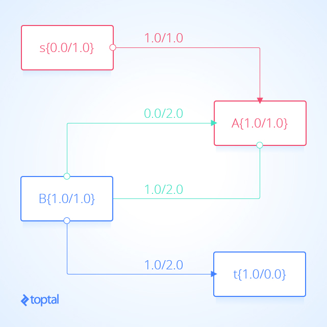
Here’s a visualization of a mfps along with its associated maxFlowProb . Each arc a in the image has a label, these labels are a.datum.flowFrom / a.datum.flowTo , each node n in the image has a label, and these labels are n.uid {n.datum.flowIn / a.datum.flowOut} .
s-t Cut Flow
Let mfps represent a MaxFlowProblemState and let stCut represent a cut of mfps.G . The cut flow of stCut is defined:
s-t cut flow is the sum of flows from the partition containing the source node to the partition containing the terminal node minus the sum of flows from the partition containing the terminal node to the partition containing the source node .
Max Flow, Min Cut
Let maxFlowProblem represent a maximum flow problem and let the solution to maxFlowProblem be represented by a flow network represented as digraph H .
Let minStCut be the minimum capacity cut of the flow network represented by maxFlowProblem.G .
Because in the maximum flow problem flow originates in only a single source node and terminates at a single terminal node and, because of the capacity constraints and the conservation constraints , we know that the all of the flow entering maxFlowProblem.terminalNodeUid must cross any s-t cut , in particular it must cross minStCut . This means:
Solving the Maximum Flow Problem
The basic idea for solving a maximum flow problem maxFlowProblem is to start with a maximum flow solution represented by digraph H . Such a starting point can be H = strip_flows(maxFlowProblem.G) . The task is then to use H and by some greedy modification of the a.datum.flow values of some arcs a in H.setOfArcs to produce another maximum flow solution represented by digraph K such that K cannot still represent a flow network with feasible flows and get_flow_value(H, maxFlowProblem) < get_flow_value(K, maxFlowProblem) . As long as this process continues, the quality ( get_flow_value(K, maxFlowProblem) ) of the most recently encountered maximum flow solution ( K ) is better than any other maximum flow solution that has been found. If the process reaches a point that it knows that no other improvement is possible, the process can terminate and it will return the optimal maximum flow solution .
The description above is general and skips many proofs such as whether such a process is possible or how long it may take, I’ll give a few more details and the algorithm.
The Max Flow, Min Cut Theorem
From the book Flows in Networks by Ford and Fulkerson , the statement of the max flow, min cut theorem (Theorem 5.1) is:
For any network, the maximal flow value from s to t is equal to the minimum cut capacity of all cuts separating s and t .
Using the definitions in this post, that translates to:
The solution to a maxFlowProblem represented by a flow network represented as digraph H is optimal if:
I like this proof of the theorem and Wikipedia has another one .
The max flow, min cut theorem is used to prove the correctness and completeness of the Ford-Fulkerson method .
I’ll also give a proof of the theorem in the section after augmenting paths .
The Ford-Fulkerson Method and the Edmonds-Karp Algorithm
CLRS defines the Ford-Fulkerson method like so (section 26.2):
Residual Graph
The Residual Graph of a flow network represented as the digraph G can be represented as a digraph G_f :
agg_n_to_u_cap(n,u,G_as_dict) returns the sum of a.datum.capacity for all arcs in the subset of G.setOfArcs where arc a is in the subset if a.fromNode = n and a.toNode = u .
agg_n_to_u_cap(n,u,G_as_dict) returns the sum of a.datum.flow for all arcs in the subset of G.setOfArcs where arc a is in the subset if a.fromNode = n and a.toNode = u .
Briefly, the residual graph G_f represents certain actions which can be performed on the digraph G .
Each pair of nodes n,u in G.setOfNodes of the flow network represented by digraph G can generate 0, 1, or 2 arcs in the residual graph G_f of G .
The pair n,u does not generate any arcs in G_f if there is no arc a in G.setOfArcs such that a.fromNode = n and a.toNode = u .
The pair n,u generates the arc a in G_f.setOfArcs where a represents an arc labeled a push flow arc from n to u a = Arc(n,u,datum=ResidualNode(n_to_u_cap_sum - n_to_u_flow_sum)) if n_to_u_cap_sum > n_to_u_flow_sum .
The pair n,u generates the arc a in G_f.setOfArcs where a represents an arc labeled a pull flow arc from n to u a = Arc(n,u,datum=ResidualNode(n_to_u_cap_sum - n_to_u_flow_sum)) if n_to_u_flow_sum > 0.0 .
Each push flow arc in G_f.setOfArcs represents the action of adding a total of x <= n_to_u_cap_sum - n_to_u_flow_sum flow to arcs in the subset of G.setOfArcs where arc a is in the subset if a.fromNode = n and a.toNode = u .
Each pull flow arc in G_f.setOfArcs represents the action of subtracting a total of x <= n_to_u_flow_sum flow to arcs in the subset of G.setOfArcs where arc a is in the subset if a.fromNode = n and a.toNode = u .
Performing an individual push or pull action from G_f on the applicable arcs in G might generate a flow network without feasible flows because the capacity constraints or the conservation constraints might be violated in the generated flow network .
Here’s a visualization of the residual graph of the previous example visualization of a maximum flow solution , in the visualization each arc a represents a.residualCapacity .
Augmenting Path
Let maxFlowProblem be a max flow problem , and let G_f = get_residual_graph_of(G) be the residual graph of maxFlowProblem.G .
An augmenting path augmentingPath for maxFlowProblem is any path from find_node_by_uid(maxFlowProblem.sourceNode,G_f) to find_node_by_uid(maxFlowProblem.terminalNode,G_f) .
It turns out that an augmenting path augmentingPath can be applied to a max flow solution represented by digraph H generating another max flow solution represented by digraph K where get_flow_value(H, maxFlowProblem) < get_flow_value(K, maxFlowProblem) if H is not optimal .
Here’s how:
In the above, TOL is some tolerance value for rounding the flow values in the network. This is to avoid cascading imprecision of floating point calculations . So, for example, I used TOL = 10 to mean round to 10 significant digits .
Let K = augment(augmentingPath, H) , then K represents a feasible max flow solution for maxFlowProblem . For the statement to be true, the flow network represented by K must have feasible flows (not violate the capacity constraint or the conservation constraint .
Here’s why: In the method above, each node added to the new flow network represented by digraph K is either an exact copy of a node from digraph H or a node n which has had the same number added to its n.datum.flowIn as its n.datum.flowOut . This means that the conservation constraint is satisfied in K as long as it was satisfied in H . The conservation constraint is satisfied because we explicitly check that any new arc a in the network has a.datum.flow <= a.datum.capacity ; thus, as long as the arcs from the set H.setOfArcs which were copied unmodified into K.setOfArcs do not violate the capacity constraint , then K does not violate the capacity constraint .
It’s also true that get_flow_value(H, maxFlowProblem) < get_flow_value(K, maxFlowProblem) if H is not optimal .
Here’s why: For an augmenting path augmentingPath to exist in the digraph representation of the residual graph G_f of a max flow problem maxFlowProblem then the last arc a on augmentingPath must be a ‘push’ arc and it must have a.toNode == maxFlowProblem.terminalNode . An augmenting path is defined as one which terminates at the terminal node of the max flow problem for which it is an augmenting path . From the definition of the residual graph , it is clear that the last arc in an augmenting path on that residual graph must be a ‘push’ arc because any ‘pull’ arc b in the augmenting path will have b.toNode == maxFlowProblem.terminalNode and b.fromNode != maxFlowProblem.terminalNode from the definition of path . Additionally, from the definition of path , it is clear that the terminal node is only modified once by the augment method. Thus augment modifies maxFlowProblem.terminalNode.flowIn exactly once and it increases the value of maxFlowProblem.terminalNode.flowIn because the last arc in the augmentingPath must be the arc which causes the modification in maxFlowProblem.terminalNode.flowIn during augment . From the definition of augment as it applies to ‘push’ arcs , the maxFlowProblem.terminalNode.flowIn can only be increased, not decreased.
Some Proofs from Sedgewick and Wayne
The book Algorithms, fourth edition by Robert Sedgewich and Kevin Wayne has some wonderful and short proofs (pages 892-894) that will be useful. I’ll recreate them here, though I’ll use language fitting in with previous definitions. My labels for the proofs are the same as in the Sedgewick book.
Proposition E: For any digraph H representing a feasible maximum flow solution to a maximum flow problem maxFlowProblem , for any stCut get_stcut_flow(stCut,H,maxFlowProblem) = get_flow_value(H, maxFlowProblem) .
Proof: Let stCut=stCut(maxFlowProblem.sourceNode,maxFlowProblem.terminalNode,set([a for a in H.setOfArcs if a.toNode == maxFlowProblem.terminalNode])) . Proposition E holds for stCut directly from the definition of s-t flow value . Suppose that there we wish to move some node n from the s-partition ( get_first_part(stCut.cut, G) ) and into the t-partition (get_second_part(stCut.cut, G)) , to do so we need to change stCut.cut , which could change stcut_flow = get_stcut_flow(stCut,H,maxFlowProblem) and invalidate proposition E . However, let’s see how the value of stcut_flow will change as we make this change. node n is at equilibrium meaning that the sum of flow into node n is equal to the sum of flow out of it (this is necessary for H to represent a feasible solution ). Notice that all flow which is part of the stcut_flow entering node n enters it from the s-partition (flow entering node n from the t-partition either directly or indirectly would not have been counted in the stcut_flow value because it is heading the wrong direction based on the definition). Additionally, all flow exiting n will eventually (directly or indirectly) flow into the terminal node (proved earlier). When we move node n into the t-partition, all the flow entering n from the s-partition must be added to the new stcut_flow value; however, all flow exiting n must the be subtracted from the new stcut_flow value; the part of the flow heading directly into the t-partition is subtracted because this flow is now internal to the new t-partition and is not counted as stcut_flow . The part of the flow from n heading into nodes in the s-partition must also be subtracted from stcut_flow : After n is moved into the t-partition, these flows will be directed from the t-partition and into the s-partition and so must not be accounted for in the stcut_flow , since these flows are removed the inflow into the s-partition and must be reduced by the sum of these flows, and the outflow from the s-partition into the t-partition (where all flows from s-t must end up) must be reduced by the same amount. As node n was at equilibrium prior to the process, the update will have added the same value to the new stcut_flow value as it subtracted thus leaving proposition E true after the update. The validity of proposition E then follows from induction on the size of the t-partition.
Here are some example flow networks to help visualize the less obvious cases where proposition E holds; in the image, the red areas indicate the s-partition, the blue areas represent the t-partition, and the green arcs indicate an s-t cut . In the second image, flow between node A and node B increases while the flow into terminal node t doesn’t change.:
Corollary: No s-t cut flow value can exceed the capacity of any s-t cut .
Proposition F. (max flow, min cut theorem): Let f be an s-t flow . The following 3 conditions are equivalent:
There exists an s-t cut whose capacity equals the value of the flow f .
f is a max flow .
There is no augmenting path with respect to f .
Condition 1 implies condition 2 by the corollary. Condition 2 implies condition 3 because the existence of an augmenting path implies the existence of a flow with larger values, contradicting the maximality of f . Condition 3 implies condition 1: Let C_s be the set of all nodes that can be reached from s with an augmenting path in the residual graph . Let C_t be the remaining arcs , then t must be in C_t (by our assumption). The arcs crossing from C_s to C_t then form an s-t cut which contains only arcs a where either a.datum.capacity = a.datum.flow or a.datum.flow = 0.0 . If this were otherwise then the nodes connected by an arc with remaining residual capacity to C_s would be in the set C_s since there would then be an augmenting path from s to such a node . The flow across the s-t cut is equal to the s-t cut’s capacity (since arcs from C_s to C_t have flow equal to capacity) and also to the value of the s-t flow (by proposition E ).
This statement of the max flow, min cut theorem implies the earlier statement from Flows in Networks .
Corollary (integrality property): When capacities are integers, there exists an integer-valued max flow, and the Ford-Fulkerson algorithm finds it.
Proof: Each augmenting path increases the flow by a positive integer, the minimum of the unused capacities in the ‘push’ arcs and the flows in the ‘pull’ arcs , all of which are always positive integers.
This justifies the Ford-Fulkerson method description from CLRS . The method is to keep finding augmenting paths and applying augment to the latest maxFlowSolution coming up with better solutions, until no more augmenting path meaning that the latest maximum flow solution is optimal .
From Ford-Fulkerson to Edmonds-Karp
The remaining questions regarding solving maximum flow problems are:
How should augmenting paths be constructed?
Will the method terminate if we use real numbers and not integers?
How long will it take to terminate (if it does)?
The Edmonds-Karp algorithm specifies that each augmenting path is constructed by a breadth first search ( BFS ) of the residual graph ; it turns out that this decision of point 1 above will also force the algorithm to terminate (point 2) and allows the asymptotic time and space complexity to be determined.
First, here’s a BFS implementation:
I used a deque from the python collections module .
To answer question 2 above, I’ll paraphrase another proof from Sedgewick and Wayne : Proposition G. The number of augmenting paths needed in the Edmonds-Karp algorithm with N nodes and A arcs is at most NA/2 . Proof: Every augmenting path has a bottleneck arc - an arc that is deleted from the residual graph because it corresponds either to a ‘push’ arc that becomes filled to capacity or a ‘pull’ arc through which the flow becomes 0. Each time an arc becomes a bottleneck arc , the length of any augmenting path through it must increase by a factor of 2. This is because each node in a path may appear only once or not at all (from the definition of path ) since the paths are being explored from shortest path to longest that means that at least one more node must be visited by the next path that goes through the particular bottleneck node that means an additional 2 arcs on the path before we arrive at the node . Since the augmenting path is of length at most N each arc can be on at most N/2 augmenting paths , and the total number of augmenting paths is at most NA/2 .
The Edmonds-Karp algorithm executes in O(NA^2) . If at most NA/2 paths will be explored during the algorithm and exploring each path with BFS is N+A then the most significant term of the product and hence the asymptotic complexity is O(NA^2) .
Let mfp be a maxFlowProblemState .
The version above is inefficient and has worse complexity than O(NA^2) since it constructs a new maximum flow solution and new a residual graph each time (rather than modifying existing digraphs as the algorithm advances). To get to a true O(NA^2) solution the algorithm must maintain both the digraph representing the maximum flow problem state and its associated residual graph . So the algorithm must avoid iterating over arcs and nodes unnecessarily and update their values and associated values in the residual graph only as necessary.
To write a faster Edmonds Karp algorithm, I rewrote several pieces of code from the above. I hope that going through the code which generated a new digraph was helpful in understanding what’s going on. In the fast algorithm, I use some new tricks and Python data structures that I don’t want to go over in detail. I will say that a.fromNode and a.toNode are now treated as strings and uids to nodes . For this code, let mfps be a maxFlowProblemState
Here’s a visualization of how this algorithm solves the example flow network from above. The visualization shows the steps as they are reflected in the digraph G representing the most up-to-date flow network and as they are reflected in the residual graph of that flow network. Augmenting paths in the residual graph are shown as red paths, and the digraph representing the problem the set of nodes and arcs affected by a given augmenting path is highlighted in green. In each case, I’ll highlight the parts of the graph that will be changed (in red or green) and then show the graph after the changes (just in black).
Here’s another visualization of how this algorithm solving a different example flow network . Notice that this one uses real numbers and contains multiple arcs with the same fromNode and toNode values.
**Also notice that because Arcs with a ‘pull’ ResidualDatum may be part of the Augmenting Path, the nodes affected in the DiGraph of the Flown Network _may not be on a path in G! .
Bipartite Graphs
Suppose we have a digraph G , G is bipartite if it’s possible to partition the nodes in G.setOfNodes into two sets ( part_1 and part_2 ) such that for any arc a in G.setOfArcs it cannot be true that a.fromNode in part_1 and a.toNode in part_1 . It also cannot be true that a.fromNode in part_2 and a.toNode in part_2 .
In other words G is bipartite if it can be partitioned into two sets of nodes such that every arc must connect a node in one set to a node in the other set.
Testing Bipartite
Suppose we have a digraph G , we want to test if it is bipartite . We can do this in O(|G.setOfNodes|+|G.setOfArcs|) by greedy coloring the graph into two colors.
First, we need to generate a new digraph H . This graph will have will have the same set of nodes as G , but it will have more arcs than G . Every arc a in G will create 2 arcs in H ; the first arc will be identical to a , and the second arc reverses the director of a ( b = Arc(a.toNode,a.fromNode,a.datum) ).
Matchings and Maximum Matchings
Suppose we have a digraph G and matching is a subset of arcs from G.setOfArcs . matching is a matching if for any two arcs a and b in matching : len(frozenset( {a.fromNode} ).union( {a.toNode} ).union( {b.fromNode} ).union( {b.toNode} )) == 4 . In other words, no two arcs in a matching share a node .
Matching matching , is a maximum matching if there is no other matching alt_matching in G such that len(matching) < len(alt_matching) . In other words, matching is a maximum matching if it is the largest set of arcs from G.setOfArcs that still satisfies the definition of matching (the addition of any arc not already in the matching will break the matching definition).
A maximum matching matching is a perfect matching if every for node n in G.setOfArcs there exists an arc a in matching where a.fromNode == n or a.toNode == n .
Maximum Bipartite Matching
A maximum bipartite matching is a maximum matching on a digraph G which is bipartite .
Given that G is bipartite , the problem of finding a maximum bipartite matching can be transformed into a maximum flow problem solvable with the Edmonds-Karp algorithm and then the maximum bipartite matching can be recovered from the solution to the maximum flow problem .
Let bipartition be a bipartition of G .
To do this, I need to generate a new digraph ( H ) with some new nodes ( H.setOfNodes ) and some new arcs ( H.setOfArcs ). H.setOfNodes contains all the nodes in G.setOfNodes and two more nodess , s (a source node ) and t (a terminal node ).
H.setOfArcs will contain one arc for each G.setOfArcs . If an arc a is in G.setOfArcs and a.fromNode is in bipartition.firstPart and a.toNode is in bipartition.secondPart then include a in H (adding a FlowArcDatum(1,0) ).
If a.fromNode is in bipartition.secondPart and a.toNode is in bipartition.firstPart , then include Arc(a.toNode,a.fromNode,FlowArcDatum(1,0)) in H.setOfArcs .
The definition of a bipartite graph ensures that no arc connects any nodes where both nodes are in the same partition. H.setOfArcs also contains an arc from node s to each node in bipartition.firstPart . Finally, H.setOfArcs contains an arc each node in bipartition.secondPart to node t . a.datum.capacity = 1 for all a in H.setOfArcs .
First partition the nodes in G.setOfNodes the two disjoint sets ( part1 and part2 ) such that no arc in G.setOfArcs is directed from one set to the same set (this partition is possible because G is bipartite ). Next, add all arcs in G.setOfArcs which are directed from part1 to part2 into H.setOfArcs . Then create a single source node s and a single terminal node t and create some more arcs
Then, construct a maxFlowProblemState .
Minimal Node Cover
A node cover in a digraph G is a set of nodes ( cover ) from G.setOfNodes such that for any arc a of G.setOfArcs this must be true: (a.fromNode in cover) or (a.toNode in cover) .
A minimal node cover is the smallest possible set of nodes in the graph that is still a node cover . König’s theorem states that in a bipartite graph, the size of the maximum matching on that graph is equal to the size of the minimal node cover , and it suggests how the node cover can recovered from a maximum matching :
Suppose we have the bipartition bipartition and the maximum matching matching . Define a new digraph H , H.setOfNodes=G.setOfNodes , the arcs in H.setOfArcs are the union of two sets.
The first set is arcs a in matching , with the change that if a.fromNode in bipartition.firstPart and a.toNode in bipartition.secondPart then a.fromNode and a.toNode are swapped in the created arc give such arcs a a.datum.inMatching=True attribute to indicate that they were derived from arcs in a matching .
The second set is arcs a NOT in matching , with the change that if a.fromNode in bipartition.secondPart and a.toNode in bipartition.firstPart then a.fromNode and a.toNode are swapped in the created arc (give such arcs a a.datum.inMatching=False attribute).
Next, run a depth first search ( DFS ) starting from each node n in bipartition.firstPart which is neither n == a.fromNode nor n == a.toNodes for any arc a in matching . During the DFS, some nodes are visited and some are not (store this information in a n.datum.visited field). The minimum node cover is the union of the nodes {a.fromNode for a in H.setOfArcs if ( (a.datum.inMatching) and (a.fromNode.datum.visited) ) } and the nodes {a.fromNode for a in H.setOfArcs if (a.datum.inMatching) and (not a.toNode.datum.visited)} .
This can be shown to lead from a maximum matching to a minimal node cover by a proof by contradiction , take some arc a that was supposedly not covered and consider all four cases regarding whether a.fromNode and a.toNode belong (whether as toNode or fromNode ) to any arc in matching matching . Each case leads to a contradiction due to the order that DFS visits nodes and the fact that matching is a maximum matching .
Suppose we have a function to execute these steps and return the set of nodes comprising the minimal node cover when given the digraph G , and the maximum matching matching :
The Linear Assignment Problem
The linear assignment problem consists of finding a maximum weight matching in a weighted bipartite graph.
Problems like the one at the very start of this post can be expressed as a linear assignment problem . Given a set of workers, a set of tasks, and a function indicating the profitability of an assignment of one worker to one task, we want to maximize the sum of all assignments that we make; this is a linear assignment problem .
Assume that the number of tasks and workers are equal, though I will show that this assumption is easy to remove. In the implementation, I represent arc weights with an attribute a.datum.weight for an arc a .
Kuhn-Munkres Algorithm
The Kuhn-Munkres Algorithm solves the linear assignment problem . A good implementation can take O(N^{4}) time, (where N is the number of nodes in the digraph representing the problem). An implementation that is easier to explain takes O(N^{5}) (for a version which regenerates DiGraphs ) and O(N^{4}) for (for a version which maintains DiGraphs ). This is similar to the two different implementations of the Edmonds-Karp algorithm.
For this description, I’m only working with complete bipartite graphs (those where half the nodes are in one part of the bipartition and the other half in the second part). In the worker, task motivation this means that there are as many workers as tasks.
This seems like a significant condition (what if these sets are not equal!) but it is easy to fix this issue; I talk about how to do that in the last section.
The version of the algorithm described here uses the useful concept of zero weight arcs . Unfortunately, this concept only makes sense when we are solving a minimization (if rather than maximizing the profits of our worker-task assignments we were instead minimizing the cost of such assignments).
Fortunately, it is easy to turn a maximum linear assignment problem into a minimum linear assignment problem by setting each the arc a weights to M-a.datum.weight where M=max({a.datum.weight for a in G.setOfArcs}) . The solution to the original maximizing problem will be identical to the solution minimizing problem after the arc weights are changed. So for the remainder, assume that we make this change.
The Kuhn-Munkres algorithm solves minimum weight matching in a weighted bipartite graph by a sequence of maximum matchings in unweighted bipartite graphs. If a we find a perfect matching on the digraph representation of the linear assignment problem , and if the weight of every arc in the matching is zero, then we have found the minimum weight matching since this matching suggests that all nodes in the digraph have been matched by an arc with the lowest possible cost (no cost can be lower than 0, based on prior definitions).
No other arcs can be added to the matching (because all nodes are already matched) and no arcs should be removed from the matching because any possible replacement arc will have at least as great a weight value.
If we find a maximum matching of the subgraph of G which contains only zero weight arcs , and it is not a perfect matching , we don’t have a full solution (since the matching is not perfect ). However, we can produce a new digraph H by changing the weights of arcs in G.setOfArcs in a way that new 0-weight arcs appear and the optimal solution of H is the same as the optimal solution of G . Since we guarantee that at least one zero weight arc is produced at each iteration, we guarantee that we will arrive at a perfect matching in no more than |G.setOfNodes|^{2}=N^{2} such iterations.
Suppose that in bipartition bipartition , bipartition.firstPart contains nodes representing workers, and bipartition.secondPart represents nodes representing tasks.
The algorithm starts by generating a new digraph H . H.setOfNodes = G.setOfNodes . Some arcs in H are generated from nodes n in bipartition.firstPart . Each such node n generates an arc b in H.setOfArcs for each arc a in bipartition.G.setOfArcs where a.fromNode = n or a.toNode = n , b=Arc(a.fromNode, a.toNode, a.datum.weight - z) where z=min(x.datum.weight for x in G.setOfArcs if ( (x.fromNode == n) or (x.toNode == n) )) .
More arcs in H are generated from nodes n in bipartition.secondPart . Each such node n generates an arc b in H.setOfArcs for each arc a in bipartition.G.setOfArcs where a.fromNode = n or a.toNode = n , b=Arc(a.fromNode, a.toNode, ArcWeightDatum(a.datum.weight - z)) where z=min(x.datum.weight for x in G.setOfArcs if ( (x.fromNode == n) or (x.toNode == n) )) .
KMA: Next, form a new digraph K composed of only the zero weight arcs from H , and the nodes incident on those arcs . Form a bipartition on the nodes in K , then use solve_mbm( bipartition ) to get a maximum matching ( matching ) on K . If matching is a perfect matching in H (the arcs in matching are incident on all nodes in H.setOfNodes ) then the matching is an optimal solution to the linear assignment problem .
Otherwise, if matching is not perfect , generate the minimal node cover of K using node_cover = get_min_node_cover(matching, bipartition(K)) . Next, define z=min({a.datum.weight for a in H.setOfArcs if a not in node_cover}) . Define nodes = H.setOfNodes , arcs1 = {Arc(a.fromNode,a.toNode,ArcWeightDatum(a.datum.weigh-z)) for a in H.setOfArcs if ( (a.fromNode not in node_cover) and (a.toNode not in node_cover)} , arcs2 = {Arc(a.fromNode,a.toNode,ArcWeightDatum(a.datum.weigh)) for a in H.setOfArcs if ( (a.fromNode not in node_cover) != (a.toNode not in node_cover)} , arcs3 = {Arc(a.fromNode,a.toNode,ArcWeightDatum(a.datum.weigh+z)) for a in H.setOfArcs if ( (a.fromNode in node_cover) and (a.toNode in node_cover)} . The != symbol in the previous expression acts as an XOR operator. Then arcs = arcs1.union(arcs2.union(arcs3)) . Next, H=DiGraph(nodes,arcs) . Go back to the label KMA . The algorithm continues until a perfect matching is produced. This matching is also the solution to the linear assignment problem .
This implementation is O(N^{5}) because it generates a new maximum matching matching at each iteration; similar to the previous two implementations of Edmonds-Karp this algorithm can be modified so that it keeps track of the matching and adapts it intelligently to each iteration. When this is done, the complexity becomes O(N^{4}) . A more advanced and more recent version of this algorithm (requiring some more advanced data structures) can run in O(N^{3}) . Details of both the simpler implementation above and the more advanced implementation can be found at this post which motivated this blog post.
None of the operations on arc weights modify the final assignment returned by the algorithm. Here’s why: Since our input graphs are always complete bipartite graphs a solution must map each node in one partition to another node in the second partition, via the arc between these two nodes . Notice that the operations performed on the arc weights never changes the order (ordered by weight) of the arcs incident on any particular node .
Thus when the algorithm terminates at a perfect complete bipartite matching each node is assigned a zero weight arc , since the relative order of the arcs from that node hasn’t changed during the algorithm, and since a zero weight arc is the cheapest possible arc and the perfect complete bipartite matching guarantees that one such arc exists for each node . This means that the solution generated is indeed the same as the solution from the original linear assignment problem without any modification of arc weights.
Unbalanced Assignments
It seems like the algorithm is quite limited since as described it operates only on complete bipartite graphs (those where half the nodes are in one part of the bipartition and the other half in the second part). In the worker, task motivation this means that there are as many workers as tasks (seems quite limiting).
However, there is an easy transformation that removes this restriction. Suppose that there are fewer workers than tasks, we add some dummy workers (enough to make the resulting graph a complete bipartite graph ). Each dummy worker has an arc directed from the worker to each of the tasks. Each such arc has weight 0 (placing it in a matching gives no added profit). After this change the graph is a complete bipartite graph which we can solve for. Any task assigned a dummy worker is not initiated.
Suppose that there are more tasks than workers. We add some dummy tasks (enough to make the resulting graph a complete bipartite graph ). Each dummy task has an arc directed from each worker to the dummy task. Each such arc has a weight of 0 (placing it in a matching gives no added profit). After this change the graph is a complete bipartite graph which we can solve for. Any worker assigned to dummy task is not employed during the period.
A Linear Assignment Example
Finally, let’s do an example with the code I’ve been using. I’m going to modify the example problem from here . We have 3 tasks: we need to clean the bathroom , sweep the floor , and wash the windows .
The workers available to use are Alice , Bob , Charlie , and Diane . Each of the workers gives us the wage they require per task. Here are the wages per worker:
| Clean the Bathroom | Sweep the Floor | Wash the Windows | |
|---|---|---|---|
| Alice | $2 | $3 | $3 |
| Bob | $3 | $2 | $3 |
| Charlie | $3 | $3 | $2 |
| Diane | $9 | $9 | $1 |
If we want to pay the least amount of money, but still get all the tasks done, who should do what task? Start by introducing a dummy task to make the digraph representing the problem bipartite.
| Clean the Bathroom | Sweep the Floor | Wash the Windows | Do Nothing | |
|---|---|---|---|---|
| Alice | $2 | $3 | $3 | $0 |
| Bob | $3 | $2 | $3 | $0 |
| Charlie | $3 | $3 | $2 | $0 |
| Diane | $9 | $9 | $1 | $0 |
Supposing that the problem is encoded in a digraph , then kuhn_munkres( bipartition(G) ) will solve the problem and return the assignment. It’s easy to verify that the optimal (lowest cost) assignment will cost $5.
Here’s a visualization of the solution the code above generates:
That is it. You now know everything you need to know about the linear assignment problem.
You can find all of the code from this article on GitHub .
Further Reading on the Toptal Blog:
- Graph Data Science With Python/NetworkX
Dmitri Ivanovich Arkhipov
Irvine, CA, United States
Member since January 23, 2017
About the author
World-class articles, delivered weekly.
By entering your email, you are agreeing to our privacy policy .
Toptal Developers
- Adobe Commerce (Magento) Developers
- Angular Developers
- AWS Developers
- Azure Developers
- Big Data Architects
- Blockchain Developers
- Business Intelligence Developers
- C Developers
- Computer Vision Developers
- Django Developers
- Docker Developers
- Elixir Developers
- Go Engineers
- GraphQL Developers
- Jenkins Developers
- Kotlin Developers
- Kubernetes Developers
- .NET Developers
- R Developers
- React Native Developers
- Ruby on Rails Developers
- Salesforce Developers
- Tableau Developers
- Unreal Engine Developers
- Xamarin Developers
- View More Freelance Developers
Join the Toptal ® community.
linear_sum_assignment #
Solve the linear sum assignment problem.
The cost matrix of the bipartite graph.
Calculates a maximum weight matching if true.
An array of row indices and one of corresponding column indices giving the optimal assignment. The cost of the assignment can be computed as cost_matrix[row_ind, col_ind].sum() . The row indices will be sorted; in the case of a square cost matrix they will be equal to numpy.arange(cost_matrix.shape[0]) .
for sparse inputs
The linear sum assignment problem [1] is also known as minimum weight matching in bipartite graphs. A problem instance is described by a matrix C, where each C[i,j] is the cost of matching vertex i of the first partite set (a ‘worker’) and vertex j of the second set (a ‘job’). The goal is to find a complete assignment of workers to jobs of minimal cost.
Formally, let X be a boolean matrix where \(X[i,j] = 1\) iff row i is assigned to column j. Then the optimal assignment has cost
where, in the case where the matrix X is square, each row is assigned to exactly one column, and each column to exactly one row.
This function can also solve a generalization of the classic assignment problem where the cost matrix is rectangular. If it has more rows than columns, then not every row needs to be assigned to a column, and vice versa.
This implementation is a modified Jonker-Volgenant algorithm with no initialization, described in ref. [2] .
Added in version 0.17.0.
https://en.wikipedia.org/wiki/Assignment_problem
DF Crouse. On implementing 2D rectangular assignment algorithms. IEEE Transactions on Aerospace and Electronic Systems , 52(4):1679-1696, August 2016, DOI:10.1109/TAES.2016.140952
- Stack Overflow for Teams Where developers & technologists share private knowledge with coworkers
- Advertising & Talent Reach devs & technologists worldwide about your product, service or employer brand
- OverflowAI GenAI features for Teams
- OverflowAPI Train & fine-tune LLMs
- Labs The future of collective knowledge sharing
- About the company Visit the blog
Collectives™ on Stack Overflow
Find centralized, trusted content and collaborate around the technologies you use most.
Q&A for work
Connect and share knowledge within a single location that is structured and easy to search.
Get early access and see previews of new features.
Which assignment algorithm should I use?
I have a single set and I need to generate pairs of two elements among this set. The assignments are all weighted. The matching shall be either constricted or perfect, depends on the results. I guess, I need a weighted matching in general graphs and, as far as I see, Edmonds's algorithm is the correct address. Is that right?
I already implemented Kuhn-Munkres algorithm but I recognized very late that this is only working on bi-partite graphs. Is there maybe a (easy) way to adjust the Kuhn-Munkres algorithm to Edmond's? Otherwise I would go for the Edmond's algorithm.
- hungarian-algorithm
- edmonds-karp
- 1 If you want to save some time, have a look at NetworkX - it already has an implementation of Edmond's algorithm : networkx.readthedocs.io/en/latest/reference/generated/… – Peter de Rivaz Commented May 21, 2017 at 21:35
- Duplicate your set and use the Hungarian algorithm on both sets with the weight of a self connection as high as possible. I haven't tried it myself, but I think it should work. – Yay295 Commented May 22, 2017 at 0:57
- @Yay295 Thanks for the advice! I already tried to double the set but this does not work.By assigning them a high weight avoids a self connection, that's correct. But problem is that elements are picked more than once because each element comes twice and the algorithm does not know that e.g. "A1" is also "B1". But I tried to implement researchgate.net/publication/… where they sate one has to "mirror" the edges - but I think the approach is wrong bc the algorithm fails often. – Ben Commented May 22, 2017 at 9:58
- 2 Cross-posted: cs.stackexchange.com/q/75751/755 , stackoverflow.com/q/44101959/781723 . Please do not post the same question on multiple sites . Each community should have an honest shot at answering without anybody's time being wasted. – D.W. Commented May 22, 2017 at 16:28
- 1 @Ben, yup, I am familiar with the difference between the two sites. That doesn't change the fact that cross-posting is prohibited. You can follow the link I gave you to learn more. You have copy-pasted your question word-for-word identical on both sites. If you want to ask about the theory part on one site, and the practice part on another site, at a minimum I would think that would require the two questions to be different, so we know what specifically you are asking. – D.W. Commented May 22, 2017 at 17:29
Know someone who can answer? Share a link to this question via email , Twitter , or Facebook .
Your answer.
Reminder: Answers generated by artificial intelligence tools are not allowed on Stack Overflow. Learn more
Sign up or log in
Post as a guest.
Required, but never shown
By clicking “Post Your Answer”, you agree to our terms of service and acknowledge you have read our privacy policy .
Browse other questions tagged algorithm matching hungarian-algorithm edmonds-karp or ask your own question .
- The Overflow Blog
- The hidden cost of speed
- The creator of Jenkins discusses CI/CD and balancing business with open source
- Featured on Meta
- Announcing a change to the data-dump process
- Bringing clarity to status tag usage on meta sites
- What does a new user need in a homepage experience on Stack Overflow?
- Feedback requested: How do you use tag hover descriptions for curating and do...
- Staging Ground Reviewer Motivation
Hot Network Questions
- What's the purpose of scanning the area before opening the portal?
- What prevents random software installation popups from mis-interpreting our consents
- How to go from Asia to America by ferry
- What is the missing fifth of the missing fifths?
- What was IBM VS/PC?
- What's the best format or way to generate a short-lived access token?
- Humans are forbidden from using complex computers. But what defines a complex computer?
- Understanding the parabolic state of a quantum particle in the infinite square well
- How can we know how good a TRNG is?
- I want to be a observational astronomer, but have no idea where to start
- Has anyone returned from space in a different vehicle from the one they went up in? And if so who was the first?
- Applying to faculty jobs in universities without a research group in your area
- Setting the desired kernel in GRUB menu
- How to clean a female disconnect connector
- How to simplify input to a table with many columns?
- Background package relying on obsolete everypage package
- The head of a screw is missing on one side of the spigot outdoor
- Is reading sheet music difficult?
- Starting with 2014 "+" signs and 2015 "−" signs, you delete signs until one remains. What’s left?
- Minimal permutation degree of the dihedral group
- Which volcano is more hazardous? Mount Rainier or Mount Hood?
- Can the canonical Eudoxus-real representatives be defined easily?
- Beatles reference in parody story from the 1980s
- Why a minus sign is often put into the law of induction for an inductor
- Kuhn's algorithm
- Running time
- Practice Problems
- Hungarian Algorithm
Kuhn's Algorithm for Maximum Bipartite Matching 
Problem ¶.
You are given a bipartite graph $G$ containing $n$ vertices and $m$ edges. Find the maximum matching, i.e., select as many edges as possible so that no selected edge shares a vertex with any other selected edge.
Algorithm Description 
Required definitions ¶.
A matching $M$ is a set of pairwise non-adjacent edges of a graph (in other words, no more than one edge from the set should be incident to any vertex of the graph $M$ ). The cardinality of a matching is the number of edges in it. All those vertices that have an adjacent edge from the matching (i.e., which have degree exactly one in the subgraph formed by $M$ ) are called saturated by this matching.
A maximal matching is a matching $M$ of a graph $G$ that is not a subset of any other matching.
A maximum matching (also known as maximum-cardinality matching) is a matching that contains the largest possible number of edges. Every maximum matching is a maximal matching.
A path of length $k$ here means a simple path (i.e. not containing repeated vertices or edges) containing $k$ edges, unless specified otherwise.
An alternating path (in a bipartite graph, with respect to some matching) is a path in which the edges alternately belong / do not belong to the matching.
An augmenting path (in a bipartite graph, with respect to some matching) is an alternating path whose initial and final vertices are unsaturated, i.e., they do not belong in the matching.
The symmetric difference (also known as the disjunctive union ) of sets $A$ and $B$ , represented by $A \oplus B$ , is the set of all elements that belong to exactly one of $A$ or $B$ , but not to both. That is, $A \oplus B = (A - B) \cup (B - A) = (A \cup B) - (A \cap B)$ .
Berge's lemma 
This lemma was proven by the French mathematician Claude Berge in 1957, although it already was observed by the Danish mathematician Julius Petersen in 1891 and the Hungarian mathematician Denés Kőnig in 1931.
Formulation 
A matching $M$ is maximum $\Leftrightarrow$ there is no augmenting path relative to the matching $M$ .
Proof 
Both sides of the bi-implication will be proven by contradiction.
A matching $M$ is maximum $\Rightarrow$ there is no augmenting path relative to the matching $M$ .
Let there be an augmenting path $P$ relative to the given maximum matching $M$ . This augmenting path $P$ will necessarily be of odd length, having one more edge not in $M$ than the number of edges it has that are also in $M$ . We create a new matching $M'$ by including all edges in the original matching $M$ except those also in the $P$ , and the edges in $P$ that are not in $M$ . This is a valid matching because the initial and final vertices of $P$ are unsaturated by $M$ , and the rest of the vertices are saturated only by the matching $P \cap M$ . This new matching $M'$ will have one more edge than $M$ , and so $M$ could not have been maximum.
Formally, given an augmenting path $P$ w.r.t. some maximum matching $M$ , the matching $M' = P \oplus M$ is such that $|M'| = |M| + 1$ , a contradiction.
A matching $M$ is maximum $\Leftarrow$ there is no augmenting path relative to the matching $M$ .
Let there be a matching $M'$ of greater cardinality than $M$ . We consider the symmetric difference $Q = M \oplus M'$ . The subgraph $Q$ is no longer necessarily a matching. Any vertex in $Q$ has a maximum degree of $2$ , which means that all connected components in it are one of the three -
- an isolated vertex
- a (simple) path whose edges are alternately from $M$ and $M'$
- a cycle of even length whose edges are alternately from $M$ and $M'$
Since $M'$ has a cardinality greater than $M$ , $Q$ has more edges from $M'$ than $M$ . By the Pigeonhole principle, at least one connected component will be a path having more edges from $M'$ than $M$ . Because any such path is alternating, it will have initial and final vertices unsaturated by $M$ , making it an augmenting path for $M$ , which contradicts the premise. $\blacksquare$
Kuhn's algorithm 
Kuhn's algorithm is a direct application of Berge's lemma. It is essentially described as follows:
First, we take an empty matching. Then, while the algorithm is able to find an augmenting path, we update the matching by alternating it along this path and repeat the process of finding the augmenting path. As soon as it is not possible to find such a path, we stop the process - the current matching is the maximum.
It remains to detail the way to find augmenting paths. Kuhn's algorithm simply searches for any of these paths using depth-first or breadth-first traversal. The algorithm looks through all the vertices of the graph in turn, starting each traversal from it, trying to find an augmenting path starting at this vertex.
The algorithm is more convenient to describe if we assume that the input graph is already split into two parts (although, in fact, the algorithm can be implemented in such a way that the input graph is not explicitly split into two parts).
The algorithm looks at all the vertices $v$ of the first part of the graph: $v = 1 \ldots n_1$ . If the current vertex $v$ is already saturated with the current matching (i.e., some edge adjacent to it has already been selected), then skip this vertex. Otherwise, the algorithm tries to saturate this vertex, for which it starts a search for an augmenting path starting from this vertex.
The search for an augmenting path is carried out using a special depth-first or breadth-first traversal (usually depth-first traversal is used for ease of implementation). Initially, the depth-first traversal is at the current unsaturated vertex $v$ of the first part. Let's look through all edges from this vertex. Let the current edge be an edge $(v, to)$ . If the vertex $to$ is not yet saturated with matching, then we have succeeded in finding an augmenting path: it consists of a single edge $(v, to)$ ; in this case, we simply include this edge in the matching and stop searching for the augmenting path from the vertex $v$ . Otherwise, if $to$ is already saturated with some edge $(to, p)$ , then will go along this edge: thus we will try to find an augmenting path passing through the edges $(v, to),(to, p), \ldots$ . To do this, simply go to the vertex $p$ in our traversal - now we try to find an augmenting path from this vertex.
So, this traversal, launched from the vertex $v$ , will either find an augmenting path, and thereby saturate the vertex $v$ , or it will not find such an augmenting path (and, therefore, this vertex $v$ cannot be saturated).
After all the vertices $v = 1 \ldots n_1$ have been scanned, the current matching will be maximum.
Running time 
Kuhn's algorithm can be thought of as a series of $n$ depth/breadth-first traversal runs on the entire graph. Therefore, the whole algorithm is executed in time $O(nm)$ , which in the worst case is $O(n^3)$ .
However, this estimate can be improved slightly. It turns out that for Kuhn's algorithm, it is important which part of the graph is chosen as the first and which as the second. Indeed, in the implementation described above, the depth/breadth-first traversal starts only from the vertices of the first part, so the entire algorithm is executed in time $O(n_1m)$ , where $n_1$ is the number of vertices of the first part. In the worst case, this is $O(n_1 ^ 2 n_2)$ (where $n_2$ is the number of vertices of the second part). This shows that it is more profitable when the first part contains fewer vertices than the second. On very unbalanced graphs (when $n_1$ and $n_2$ are very different), this translates into a significant difference in runtimes.
Implementation 
Standard implementation ¶.
Let us present here an implementation of the above algorithm based on depth-first traversal and accepting a bipartite graph in the form of a graph explicitly split into two parts. This implementation is very concise, and perhaps it should be remembered in this form.
Here $n$ is the number of vertices in the first part, $k$ - in the second part, $g[v]$ is the list of edges from the top of the first part (i.e. the list of numbers of the vertices to which these edges lead from $v$ ). The vertices in both parts are numbered independently, i.e. vertices in the first part are numbered $1 \ldots n$ , and those in the second are numbered $1 \ldots k$ .
Then there are two auxiliary arrays: $\rm mt$ and $\rm used$ . The first - $\rm mt$ - contains information about the current matching. For convenience of programming, this information is contained only for the vertices of the second part: $\textrm{mt[} i \rm]$ - this is the number of the vertex of the first part connected by an edge with the vertex $i$ of the second part (or $-1$ , if no matching edge comes out of it). The second array is $\rm used$ : the usual array of "visits" to the vertices in the depth-first traversal (it is needed just so that the depth-first traversal does not enter the same vertex twice).
A function $\textrm{try_kuhn}$ is a depth-first traversal. It returns $\rm true$ if it was able to find an augmenting path from the vertex $v$ , and it is considered that this function has already performed the alternation of matching along the found chain.
Inside the function, all the edges outgoing from the vertex $v$ of the first part are scanned, and then the following is checked: if this edge leads to an unsaturated vertex $to$ , or if this vertex $to$ is saturated, but it is possible to find an increasing chain by recursively starting from $\textrm{mt[}to \rm ]$ , then we say that we have found an augmenting path, and before returning from the function with the result $\rm true$ , we alternate the current edge: we redirect the edge adjacent to $to$ to the vertex $v$ .
The main program first indicates that the current matching is empty (the list $\rm mt$ is filled with numbers $-1$ ). Then the vertex $v$ of the first part is searched by $\textrm{try_kuhn}$ , and a depth-first traversal is started from it, having previously zeroed the array $\rm used$ .
It is worth noting that the size of the matching is easy to get as the number of calls $\textrm{try_kuhn}$ in the main program that returned the result $\rm true$ . The desired maximum matching itself is contained in the array $\rm mt$ .
We repeat once again that Kuhn's algorithm is easy to implement in such a way that it works on graphs that are known to be bipartite, but their explicit splitting into two parts has not been given. In this case, it will be necessary to abandon the convenient division into two parts, and store all the information for all vertices of the graph. For this, an array of lists $g$ is now specified not only for the vertices of the first part, but for all the vertices of the graph (of course, now the vertices of both parts are numbered in a common numbering - from $1$ to $n$ ). Arrays $\rm mt$ and are $\rm used$ are now also defined for the vertices of both parts, and, accordingly, they need to be kept in this state.
Improved implementation 
Let us modify the algorithm as follows. Before the main loop of the algorithm, we will find an arbitrary matching by some simple algorithm (a simple heuristic algorithm ), and only then we will execute a loop with calls to the $\textrm{try_kuhn}()$ function, which will improve this matching. As a result, the algorithm will work noticeably faster on random graphs - because in most graphs, you can easily find a matching of a sufficiently large size using heuristics, and then improve the found matching to the maximum using the usual Kuhn's algorithm. Thus, we will save on launching a depth-first traversal from those vertices that we have already included using the heuristic into the current matching.
For example, you can simply iterate over all the vertices of the first part, and for each of them, find an arbitrary edge that can be added to the matching, and add it. Even such a simple heuristic can speed up Kuhn's algorithm several times.
Please note that the main loop will have to be slightly modified. Since when calling the function $\textrm{try_kuhn}$ in the main loop, it is assumed that the current vertex is not yet included in the matching, you need to add an appropriate check.
In the implementation, only the code in the $\textrm{main}()$ function will change:
Another good heuristic is as follows. At each step, it will search for the vertex of the smallest degree (but not isolated), select any edge from it and add it to the matching, then remove both these vertices with all incident edges from the graph. Such greed works very well on random graphs; in many cases it even builds the maximum matching (although there is a test case against it, on which it will find a matching that is much smaller than the maximum).
Notes 
- Kuhn's algorithm is a subroutine in the Hungarian algorithm , also known as the Kuhn-Munkres algorithm .
- Kuhn's algorithm runs in $O(nm)$ time. It is generally simple to implement, however, more efficient algorithms exist for the maximum bipartite matching problem - such as the Hopcroft-Karp-Karzanov algorithm , which runs in $O(\sqrt{n}m)$ time.
- The minimum vertex cover problem is NP-hard for general graphs. However, Kőnig's theorem gives that, for bipartite graphs, the cardinality of the maximum matching equals the cardinality of the minimum vertex cover. Hence, we can use maximum bipartite matching algorithms to solve the minimum vertex cover problem in polynomial time for bipartite graphs.
Practice Problems 
- Kattis - Gopher II
- Kattis - Borders
- ameya-dubey (81.97%)
- Jakob Kogler (9.87%)
- Oleksandr Kulkov (5.15%)
- matbensch (2.58%)
- Eric Pei (0.43%)
IEEE Account
- Change Username/Password
- Update Address
Purchase Details
- Payment Options
- Order History
- View Purchased Documents
Profile Information
- Communications Preferences
- Profession and Education
- Technical Interests
- US & Canada: +1 800 678 4333
- Worldwide: +1 732 981 0060
- Contact & Support
- About IEEE Xplore
- Accessibility
- Terms of Use
- Nondiscrimination Policy
- Privacy & Opting Out of Cookies
A not-for-profit organization, IEEE is the world's largest technical professional organization dedicated to advancing technology for the benefit of humanity. © Copyright 2024 IEEE - All rights reserved. Use of this web site signifies your agreement to the terms and conditions.
IMAGES
VIDEO
COMMENTS
The Hungarian matching algorithm, also called the Kuhn-Munkres algorithm, is a \(O\big(|V|^3\big)\) algorithm that can be used to find maximum-weight matchings in bipartite graphs, which is sometimes called the assignment problem.A bipartite graph can easily be represented by an adjacency matrix, where the weights of edges are the entries.Thinking about the graph in terms of an adjacency ...
Matching Algorithms (Graph Theory)
Hungarian Algorithm for Assignment Problem | Set 1 ...
Lecture 8: Assignment Algorithms - Cyberlab Research
The algorithm maintains a matching M and compatible prices p. Pf. Follows from Lemmas 2 and 3 and initial choice of prices. ! Theorem. The algorithm returns a min cost perfect matching. Pf. Upon termination M is a perfect matching, and p are compatible Optimality follows from Observation 2. ! Theorem. The algorithm can be implemented in O(n 3 ...
This problem is also called the assignment problem. Similar problems (but more complicated) can be de ned on non-bipartite graphs. 1. Lecture notes on bipartite matching February 2nd, 2013 2 ... Moreover, jCj= jM jwhere M is the matching returned by the algorithm. This claim immediately proves K onig's theorem. Proof: We rst show that C is a ...
1. Application: Max Bipartite Matching A graph G = (V,E)is bipartite if there exists partition V = X ∪ Y with X ∩ Y = ∅ and E ⊆ X × Y. A Matching is a subset M ⊆ E such that ∀v ∈ V at most one edge in M is incident upon v. The size of a matching is |M|, the number of edges in M. A Maximum Matching is matching M such that every ...
Hungarian algorithm for solving the assignment problem
The graph G is bipartite if the node set V can be partitioned into two disjoint sets V 1 and V 2 such that no edge in E connects nodes from the same set. Finding a maximum cardinality matching on a bipartite graph can be solved by several efficient algorithms with a worst-case bound of \( O(\sqrt{n}m) \), where n is the number of nodes and m the number of edges of the graph.
General description of the algorithm. This problem is known as the assignment problem. The assignment problem is a special case of the transportation problem, which in turn is a special case of the min-cost flow problem, so it can be solved using algorithms that solve the more general cases. Also, our problem is a special case of binary integer ...
Assignment problem
The Hungarian method is a combinatorial optimization algorithm that solves the assignment problem in polynomial time and which anticipated later primal-dual methods.It was developed and published in 1955 by Harold Kuhn, who gave it the name "Hungarian method" because the algorithm was largely based on the earlier works of two Hungarian mathematicians, Dénes Kőnig and Jenő Egerváry.
The Dynamic Hungarian Algorithm for the Assignment ...
For implementing the above algorithm, the idea is to use the max_cost_assignment() function defined in the dlib library. This function is an implementation of the Hungarian algorithm (also known as the Kuhn-Munkres algorithm) which runs in O(N 3) time. It solves the optimal assignment problem. Below is the implementation of the above approach:
The Hungarian matching algorithm is a combinatorial optimization algorithm that solves the assignment linear-programming problem in polynomial time. The assignment problem is an interesting problem and the Hungarian algorithm is difficult to understand. In this blog post, I would like to talk about what assignment is and give some intuitions ...
women, find a stable matching. Gale-Shapley algorithm. Finds a stable matching in O(n 2) time. Man-optimality. In version of GS where men propose, each man receives best valid partner. Q. Does man-optimality come at the expense of the women? no man and woman prefer to be with each other than assigned partner w is a valid partner of m if there ...
Here, the contractors and the contracts can be modeled as a bipartite graph, with their effectiveness as the weights of the edges between the contractor and the contract nodes. In this article, you will learn about an implementation of the Hungarian algorithm that uses the Edmonds-Karp algorithm to solve the linear assignment problem.
The Hungarian method is a combinatorial optimization algorithm which solves the assignment problem in polynomial time . Later it was discovered that it was a primal-dual Simplex method.. It was developed and published by Harold Kuhn in 1955, who gave the name "Hungarian method" because the algorithm was largely based on the earlier works of two Hungarian mathematicians: Denes Konig and Jeno ...
The Hungarian Method: The following algorithm applies the above theorem to a given n × n cost matrix to find an optimal assignment. Step 1. Subtract the smallest entry in each row from all the entries of its row. Step 2. Subtract the smallest entry in each column from all the entries of its column. Step 3.
The linear sum assignment problem [1] is also known as minimum weight matching in bipartite graphs. A problem instance is described by a matrix C, where each C [i,j] is the cost of matching vertex i of the first partite set (a 'worker') and vertex j of the second set (a 'job'). The goal is to find a complete assignment of workers to ...
Matching (graph theory)
The assignments are all weighted. The matching shall be either constricted or perfect, depends on the results. I guess, I need a weighted matching in general graphs and, as far as I see, Edmonds's algorithm is the correct address. ... Matching algorithms in R (bipartite matching, Hungarian algorithm) 4
Kuhn's Algorithm - Maximum Bipartite Matching
A Gravity-Aided Navigation Matching Algorithm Based on Triangulation Abstract: Gravity aided inertial navigation system is one of the key technologies in underwater navigation. Traditional gravity background field is usually composed of gravity anomaly values measured by gravity sensors, which is in the form of grid and obviously hide the rich ...