what is matching hypothesis

12.7 Prosocial Behavior

Learning objectives.

By the end of this section, you will be able to:

• Describe altruism
• Describe conditions that influence the formation of relationships
• Identify what attracts people to each other
• Describe the triangular theory of love
• Explain social exchange theory in relationships

You’ve learned about many of the negative behaviors of social psychology, but the field also studies many positive social interactions and behaviors. What makes people like each other? With whom are we friends? Whom do we date? Researchers have documented several features of the situation that influence whether we form relationships with others. There are also universal traits that humans find attractive in others. In this section we discuss conditions that make forming relationships more likely, what we look for in friendships and romantic relationships, the different types of love, and a theory explaining how our relationships are formed, maintained, and terminated.

Prosocial Behavior and Altruism

Do you voluntarily help others? Voluntary behavior with the intent to help other people is called prosocial behavior . Why do people help other people? Is personal benefit such as feeling good about oneself the only reason people help one another? Research suggests there are many other reasons. Altruism is people’s desire to help others even if the costs outweigh the benefits of helping. In fact, people acting in altruistic ways may disregard the personal costs associated with helping ( Figure 12.26 ). For example, news accounts of the 9/11 terrorist attacks on the World Trade Center in New York reported an employee in the first tower helped his co-workers make it to the exit stairwell. After helping a co-worker to safety he went back in the burning building to help additional co-workers. In this case the costs of helping were great, and the hero lost his life in the destruction (Stewart, 2002).

Some researchers suggest that altruism operates on empathy. Empathy is the capacity to understand another person’s perspective, to feel what they feel. An empathetic person makes an emotional connection with others and feels compelled to help (Batson, 1991). Other researchers argue that altruism is a form of selfless helping that is not motivated by benefits or feeling good about oneself. Certainly, after helping, people feel good about themselves, but some researchers argue that this is a consequence of altruism, not a cause. Other researchers argue that helping is always self-serving because our egos are involved, and we receive benefits from helping (Cialdini, Brown, Lewis, Luce, & Neuberg 1997). It is challenging to determine experimentally the true motivation for helping, whether it is largely self-serving (egoism) or selfless (altruism). Thus, a debate on whether pure altruism exists continues.

Link to Learning

See this excerpt from the popular TV series Friends in which egoism versus altruism is debated to learn more.

Forming Relationships

What do you think is the single most influential factor in determining with whom you become friends and with whom you form romantic relationships? You might be surprised to learn that the answer is simple: the people with whom you have the most contact. This most important factor is proximity. You are more likely to be friends with people you have regular contact with. For example, there are decades of research that shows that you are more likely to become friends with people who live in your dorm, your apartment building, or your immediate neighborhood than with people who live farther away (Festinger, Schachler, & Back, 1950). It is simply easier to form relationships with people you see often because you have the opportunity to get to know them.

Similarity is another factor that influences who we form relationships with. We are more likely to become friends or lovers with someone who is similar to us in background, attitudes, and lifestyle. In fact, there is no evidence that opposites attract. Rather, we are attracted to people who are most like us ( Figure 12.27 ) (McPherson, Smith-Lovin, & Cook, 2001). Why do you think we are attracted to people who are similar to us? Sharing things in common will certainly make it easy to get along with others and form connections. When you and another person share similar music taste, hobbies, food preferences, and so on, deciding what to do with your time together might be easy. Homophily is the tendency for people to form social networks, including friendships, marriage, business relationships, and many other types of relationships, with others who are similar (McPherson et al., 2001).

But, homophily limits our exposure to diversity (McPherson et al., 2001). By forming relationships only with people who are similar to us, we will have homogenous groups and will not be exposed to different points of view. In other words, because we are likely to spend time with those who are most like ourselves, we will have limited exposure to those who are different than ourselves, including people of different races, ethnicities, social-economic status, and life situations.

Once we form relationships with people, we desire reciprocity. Reciprocity is the give and take in relationships. We contribute to relationships, but we expect to receive benefits as well. That is, we want our relationships to be a two way street. We are more likely to like and engage with people who like us back. Self-disclosure is part of the two way street. Self-disclosure is the sharing of personal information (Laurenceau, Barrett, & Pietromonaco, 1998). We form more intimate connections with people with whom we disclose important information about ourselves. Indeed, self-disclosure is a characteristic of healthy intimate relationships, as long as the information disclosed is consistent with our own views (Cozby, 1973).

We have discussed how proximity and similarity lead to the formation of relationships, and that reciprocity and self-disclosure are important for relationship maintenance. But, what features of a person do we find attractive? We don’t form relationships with everyone that lives or works near us, so how is it that we decide which specific individuals we will select as friends and lovers?

Researchers have documented several characteristics that humans find attractive. First we look for friends and lovers who are physically attractive. People differ in what they consider attractive, and attractiveness is culturally influenced. Research, however, suggests that some universally attractive features in women include large eyes, high cheekbones, a narrow jaw line, a slender build (Buss, 1989), and a lower waist-to-hip ratio (Singh, 1993). For men, attractive traits include being tall, having broad shoulders, and a narrow waist (Buss, 1989). Both men and women with high levels of facial and body symmetry are generally considered more attractive than asymmetric individuals (Fink, Neave, Manning, & Grammer, 2006; Penton-Voak et al., 2001; Rikowski & Grammer, 1999). Social traits that people find attractive in potential female mates include warmth, affection, and social skills; in males, the attractive traits include achievement, leadership qualities, and job skills (Regan & Berscheid, 1997). Although humans want mates who are physically attractive, this does not mean that we look for the most attractive person possible. In fact, this observation has led some to propose what is known as the matching hypothesis which asserts that people tend to pick someone they view as their equal in physical attractiveness and social desirability (Taylor, Fiore, Mendelsohn, & Cheshire, 2011). For example, you and most people you know likely would say that a very attractive movie star is out of your league. So, even if you had proximity to that person, you likely would not ask them out on a date because you believe you likely would be rejected. People weigh a potential partner’s attractiveness against the likelihood of success with that person. If you think you are particularly unattractive (even if you are not), you likely will seek partners that are fairly unattractive (that is, unattractive in physical appearance or in behavior).

Sternberg’s Triangular Theory of Love

We typically love the people with whom we form relationships, but the type of love we have for our family, friends, and lovers differs. Robert Sternberg (1986) proposed that there are three components of love: intimacy, passion, and commitment. These three components form a triangle that defines multiple types of love: this is known as Sternberg’s triangular theory of love ( Figure 12.28 ). Intimacy is the sharing of details and intimate thoughts and emotions. Passion is the physical attraction—the flame in the fire. Commitment is standing by the person—the “in sickness and health” part of the relationship.

Sternberg (1986) states that a healthy relationship will have all three components of love—intimacy, passion, and commitment—which is described as consummate love ( Figure 12.29 ). However, different aspects of love might be more prevalent at different life stages. Other forms of love include liking, which is defined as having intimacy but no passion or commitment. Infatuation is the presence of passion without intimacy or commitment. Empty love is having commitment without intimacy or passion. Companionate love , which is characteristic of close friendships and family relationships, consists of intimacy and commitment but no passion. Romantic love is defined by having passion and intimacy, but no commitment. Finally, fatuous love is defined by having passion and commitment, but no intimacy, such as a long term sexual love affair. Can you describe other examples of relationships that fit these different types of love?

Social Exchange Theory

We have discussed why we form relationships, what attracts us to others, and different types of love. But what determines whether we are satisfied with and stay in a relationship? One theory that provides an explanation is social exchange theory. According to social exchange theory , we act as naïve economists in keeping a tally of the ratio of costs and benefits of forming and maintaining a relationship with others ( Figure 12.30 ) (Rusbult & Van Lange, 2003).

People are motivated to maximize the benefits of social exchanges, or relationships, and minimize the costs. People prefer to have more benefits than costs, or to have nearly equal costs and benefits, but most people are dissatisfied if their social exchanges create more costs than benefits. Let’s discuss an example. If you have ever decided to commit to a romantic relationship, you probably considered the advantages and disadvantages of your decision. What are the benefits of being in a committed romantic relationship? You may have considered having companionship, intimacy, and passion, but also being comfortable with a person you know well. What are the costs of being in a committed romantic relationship? You may think that over time boredom from being with only one person may set in; moreover, it may be expensive to share activities such as attending movies and going to dinner. However, the benefits of dating your romantic partner presumably outweigh the costs, or you wouldn’t continue the relationship.

As an Amazon Associate we earn from qualifying purchases.

This book may not be used in the training of large language models or otherwise be ingested into large language models or generative AI offerings without OpenStax's permission.

Want to cite, share, or modify this book? This book uses the Creative Commons Attribution License and you must attribute OpenStax.

Access for free at https://openstax.org/books/psychology-2e/pages/1-introduction

• Authors: Rose M. Spielman, William J. Jenkins, Marilyn D. Lovett
• Publisher/website: OpenStax
• Book title: Psychology 2e
• Publication date: Apr 22, 2020
• Location: Houston, Texas
• Book URL: https://openstax.org/books/psychology-2e/pages/1-introduction
• Section URL: https://openstax.org/books/psychology-2e/pages/12-7-prosocial-behavior

© Jan 6, 2024 OpenStax. Textbook content produced by OpenStax is licensed under a Creative Commons Attribution License . The OpenStax name, OpenStax logo, OpenStax book covers, OpenStax CNX name, and OpenStax CNX logo are not subject to the Creative Commons license and may not be reproduced without the prior and express written consent of Rice University.

Relationship Theories Revision Notes

Will Goulder

Psychology A-level Teacher

BSc (Hons), Psychology

Psychology and performing arts teacher in Canterbury. Deputy head of language and arts, and digital technology leader.

Learn about our Editorial Process

Saul Mcleod, PhD

Editor-in-Chief for Simply Psychology

BSc (Hons) Psychology, MRes, PhD, University of Manchester

Saul Mcleod, PhD., is a qualified psychology teacher with over 18 years of experience in further and higher education. He has been published in peer-reviewed journals, including the Journal of Clinical Psychology.

On This Page:

What do the examiners look for?

• Accurate and detailed knowledge
• Clear, coherent, and focused answers
• Effective use of terminology (use the “technical terms”)

In application questions, examiners look for “effective application to the scenario,” which means that you need to describe the theory and explain the scenario using the theory making the links between the two very clear. If there is more than one individual in the scenario you must mention all of the characters to get to the top band.

Difference between AS and A level answers

The descriptions follow the same criteria; however, you have to use the issues and debates effectively in your answers. “Effectively” means that it needs to be linked and explained in the context of the answer.

Read the model answers to get a clearer idea of what is needed.

Exam Paper Advice

In the exam, you will be asked a range of questions on relationships, which may include questions about research methods or using mathematical skills based on research into relationships.

As in Paper One and Two, you may be asked a 16-mark question, which could include an item (6 marks for AO1 Description, 4 marks for AO2 Application, and 6 marks for AO3 Evaluation) or simply to discuss the topic more generally (6 marks AO1 Description and ten marks AO2 Evaluation).

There is no guarantee that a 16-mark question will be asked on this topic, though, so it is important to have a good understanding of all of the different areas linked to the topic.

There will be 24 marks for relationship questions, so you can expect to spend about 30 minutes on this section, but this is not a strict rule.

The evolutionary explanations for partner preferences

The relationship between sexual selection and human reproductive behavior.

Evolutionary approaches state that animals are motivated to select a ‘mate’ with the best possible genes who will best be able to ensure the offspring’s future health and survival.

Anisogamy means two sex cells (or gametes) that are different coming together to reproduce. Men have sperm cells, which can reproduce quickly with little energy expenditure, and once they start being produced, they do not usually stop until the man dies.

Female gametes (eggs or ova) are, in contrast, much less plentiful; they are released in a limited time frame (between puberty and menopause) and require much more energy to produce.

This difference (anisogamy) means that men and women use different strategies when choosing partners.

Inter-sexual Selection

Intersexual selection is the preferred strategy of the female. They value quality over quantity.

Intersexual selection is when one gender makes mate choices based on a specific characteristic of the other gender: e.g., peahens choosing peacocks with larger tails. As a result, peacock tails become larger across the population because peacocks with larger tails will mate more, thus passing these characteristics on.

Females lose more resources than men if they choose a sub-standard partner, so they are pickier about who they select. They are more likely to pick a partner who is genetically fit and willing to offer the maximum resources to raise their offspring (a man who will remain by her side as the child grows to protect them both and potentially provide more children).

Females tend to seek a man who displays physical health characteristics and is a high-status individual who controls resources within the social group. Thus male partners are able to protect, provide and control food and resources. Although this ability may have equated to muscular strength in our evolutionary past, in modern society, it is more likely to relate to occupation, social class, and wealth.

If they have made a good choice, then their offspring will inherit the positive features of their father and are therefore also more likely to be chosen by women or men in the next generation.

Intra-sexual Selection

Intrasexual selection is the preferred strategy of the male. They value quantity over quality. Anisogamy suggests that men’s best evolutionary strategy is to have as many partners as possible.

To succeed, men must compete with other males to present themselves as the most attractive mate, encouraging features such as muscles that indicate to the opposite sex an ability to protect both themselves and their offspring.

Intrasexual selection refers to competition between members of the same sex for access to a mate of the opposite sex. Whatever characteristics led to success in mating will be passed on to the next generation, thus becoming more widespread in the gene pool.

Buss (1989) surveyed over 10,000 adults in 33 countries and found that females reported valuing resource-based characteristics when choosing a male (such as their jobs) whilst men valued good looks and preferred younger partners more than females did.

Although the size and scale of Buss’s work are impressive, his use of questionnaires could lead to social desirability bias, with participants answering in socially desirable ways rather than honestly. Also, 77% of participants were from Western industrial nations, meaning Buss might have been measuring the effects of culture rather than an evolutionary-determined behavior.

Clark and Hatfield (1989) conducted a now infamous study where male and female psychology students were asked to approach fellow students of Florida State University (of the opposite sex) and ask them for one of three things; to go on a date, to go back to their apartment, or to go to bed with them.

About 50% of men and women agreed to the date, but 69% of men agreed to visit the apartment, and 75% agreed to go to bed with them; only 6% of women agreed to go to the apartment, and 0% accepted the more intimate offer.

The evolutionary approach is determinist suggesting that we have little free will in partner choice. However, everyday experience tells us we have some control over our preferences. Evolutionary approaches to mate preferences are socially sensitive in that they promote traditional (sexist) views regarding what are ‘natural’ male and female roles and behaviors.

Gender bias – In today’s society, women are more career orientated and, therefore,, will not look for resourceful partners as much – Evolutionary theory does not apply to modern society.

Finally, the evolutionary theory makes little attempt to explain other types of relationships, e.g., gay and lesbian relationships, and cultural variations in relationships that exist across the world, e.g., arranged marriages.

Factors Affecting Attraction

Self disclosure.

This refers to the extent to which a person reveals thoughts, feelings, and behaviors which they would usually keep private from a potential partner. This increases feelings of intimacy.

In the initial stages of a relationship, couples often seek to learn as much as they can about their new partner and feel that this sharing of information brings them closer together. But can too much sharing scare your partner away? Is not sharing very much information intriguing or frustrating?

Altman and Taylor (1973) identified breadth and depth as important factors of self-disclosure . At the start of a relationship, self-disclosure is likely to cover a range of topics as you seek to explore the key facts about your new partner. “What do you do for work” and “Where did you last go on holiday” but these topics are relatively superficial.

As the relationship develops, people tend to share more detailed and personal information, such as past traumas and desires for the future. If this sharing happens too soon, however, an incompatibility may be found before the other person has reached a suitable level of investment in the relationship. Altman and Taylor referred to this sharing of information as social penetration .

An important aspect of this is the reciprocity of the process; if one person shares more than the other is willing to, there may be a breakdown of trust as one person establishes themselves as more invested than the other.

Aron et al. (1997) found that by providing a list of questions to pairs of people that start with superficial information (Who would be your perfect dinner party guest) and moving over 36 questions to more intimate information (Of all the people in your family, whose death would you find the most disturbing) people grew closer and more intimate as the questions progressed.

Aron’s research also included a four-minute stare at the end of the question sequence, which may have also contributed to the increased intimacy.

Sprecher and Hendrick (2004) observed couples on dates and found a close correlation between the amount of satisfaction each person felt and the overall self-disclosure that occurred between the partners.

However, much of the research into self-disclosure is correlational, which means that a causal relationship cannot be easily determined; in short, it may be that it is the attraction between partners which leads to greater self-disclosure, rather than the sharing of information, that leads to greater intimacy.

Physical attractiveness: including the matching hypothesis

Physical attractiveness is viewed by society as one of the most important factors of relationship formation, but is this view supported by research?

Physical appearance can be seen as a range of indicators of underlying characteristics. Women with a favorable waist-to-hip ratio are seen as attractive because they are perceived to be more fertile (Singh, 2002), and people with more symmetrical features are seen to be more genetically fit.

This is because our genes are designed to make us develop symmetrically, but diseases and infections during physical development can cause these small imperfections and asymmetries (Little and Jones, 2003).

The halo effect is a cognitive bias (mental shortcut) that occurs when a person assumes that a person has positive traits in terms of personality and other features because they have a pleasing appearance.

Dion, Berscheid, and Walster (1972) asked participants to rate photographs of three strangers for a number of different categories, including personality traits such as overall happiness and career success.

When these results were compared to the physical attraction rating of each participant (from a rating of 100 students), the photographs which were rated the most physically attractive were also rated higher on the other positive traits.

Walster et al. proposed The Matching Hypothesis that similar people end up together. The more physically desirable someone is, the more desirable they would expect their partner to be. An individual would often choose to date a partner of approximately their own attractiveness.

The matching hypothesis (Walster et al., 1966) suggests that people realize at a young age that not everybody can form relationships with the most attractive people, so it is important to evaluate their own attractiveness and, from this, partners who are the most attainable.

If a person always went for people “out of their league” in terms of physical attractiveness, they may never find a partner, which would be evolutionarily foolish. This identification of those who have a similar level of attraction, and therefore provide a balance between the level of competition (intra-sexual) and positive traits, is referred to as matching.

Modern dating in society is increasingly visual, with the rise of online dating, particularly using apps such as Tinder.

In Dion et al.’s (1972) study, those who were rated to be the most physically attractive were not rated highly on the statement “Would be a good parent,” which could be seen to contradict theories about inter and intra-sexual selection.

Landy and Aronson (1969) show how the halo effect occurs in other contexts. They found that when victims of crime were perceived to be more attractive, defendants in court cases were more likely to be given longer sentences by a simulated jury.

When the defendants were unattractive, they were more likely to be sentenced by the jury, which supports the idea that we generalize physical attractiveness as an indicator of other, less visual traits such as trustworthiness.

Feingold (1988) conducted a meta-analysis of 17 studies and found a significant correlation between the perceived attractiveness of actual partners rated by independent participants.

Individual differences – Towhey et al. found that some people are less sensitive to physical attractiveness when making judgments of personality and likeability – The effects of physical attractiveness can be moderated by other factors and is not significant.

The Filter Theory

Kerckhoff and Davis (1962) suggested that when selecting partners from a range of those who are potentially available to them (a field of availability), people will use three filters to “narrow down” the choice to those who they have the best chance of a sustainable relationship with.

The filter model speaks about three “levels of filters” which are applied to partners.

The first filter proposed when selecting partners were social demography . Social variables such as age, social background, ethnicity, religion, etc., determine the likelihood of individuals meeting and socializing, which will, in turn, influence the likelihood of a relationship being formed.

We are also more likely to prefer potential partners with whom we share social demography as they are more similar to us, and we share more in common with them in terms of norms, attitudes, and experiences.

The second filter that Kerckhoff and Davis suggested was similarity in attitudes . Psychological variables to do with shared beliefs and attitudes are the best predictor of a relationship becoming stable. Disclosure is essential at this stage to ensure partners really do share genuine similarities.

This was supported by their original 1962 longitudinal study of two groups of student couples (those who had been together for more or less than 18 months).

Over seven months, the couples completed questionnaires based on their views and attitudes, which were then compared for similarities. Kerckhoff and Davis suggested that the similarity of attitudes was the most important factor in the group that had been together for less than 18 months. This is supported by the self-disclosure research described elsewhere on this topic.

The third filter was complementarity which goes a step further than similarity. Rather than having the same traits and attitudes, such as dominance or humor, a partner who complements their spouse has traits that the other lacks. For example, one partner may be good at organization, whilst the other is poor at the organization but very good at entertaining guests.

Kerchoff and Davis found that this level of the filter was the most important for couples who had been together for more than 18 months. This may be the origin of the classic phrase “opposites attract,” though we may add the condition “although not for the first 18 months of the relationship.

This theory may be interpreted as similar to the matching hypothesis but for personality rather than physical traits.

Some stages of this model may now be seen as less relevant; for example, as modern society is much more multicultural and interconnected (by things such as the internet) than in the 1960s, we may now see social demography as less of a barrier to a relationship. This may lead to the criticism that the theory lacks temporal validity.

This lack of temporal validity is supported by Levinger (1978), who, even only 16 years after the study, pointed out that many studies had failed to replicate Karchkoff and Davis’ original findings, although this may be down to methodological issues with operationalizing factor such as the success of a relationship or complementarity of traits.

Again, investigating the second and third levels of the filter theory looks at correlation which cannot easily explain causality. Both Davis and Rusbult (2001) and Anderson et al. (2003) found that people become more similar in different ways the more time that they spend in a relationship together.

So it may be that the relationship leads to an alignment of attitudes and also a greater complementarity as couples assign each other roles: “He does the cooking, and I do the hoovering.”

Theories of Romantic Relationships

Social exchange theory.

This is an economic theory of romantic relationships. Many psychologists believe that the key to maintaining a relationship is that it is mutually beneficial.

Psychologists Thibault and Kelley (1959) proposed the Social Exchange Theory , which stipulates that one motivation to stay in a romantic relationship, and a large factor in its development, is the result of a cost-benefit analysis that people perform, either consciously or unconsciously.

Thibaut and Kelley assume that people try to maximize the rewards they obtain from a relationship and minimize the costs (the minimax principle).

In a relationship, people gain rewards (such as attention from their partner, sex, gifts, and a boost to their self-esteem) and incur costs (paying money for gifts, compromising on how to spend their time or stress).

There is also an opportunity cost in relationships, as time spent with a partner that does not develop into a lasting relationship could have been spent with another partner with better long-term prospects.

How much value is placed on each cost and benefit is subjective and determined by the individual. For example, whilst some people may want to spend as much time as possible with their partner in the early stages of the relationship and see this time together as a reward of the relationship, others may value their space and see extended periods spent together as more of a necessary investment to keep the other person happy.

Thibault and Kelley also identified a number of different stages of a relationship which progress from the sampling stage, where couples experiment with the potential costs and rewards of a relationship through direct or indirect interactions, through the bargaining and commitment stages as negotiations of each partner’s role in the relationship occur.

The rewards and costs are established and become more predictable, and finally arriving at the institutionalization stage, where the couple is settled. The norms of the relationship are heavily embedded.

Comparison Levels (CL) and (CLalt)

The comparison level (CL) in a relationship is a judgment of how much profit an individual is receiving (benefits minus costs). The acceptable CL needed to continue to pursue a relationship changes as a person matures and can be affected by a number of external and internal factors.

External factors may include the media (younger people may want more from a relationship after being socialized by images of romance on films and television), seeing friends and families in relationships (people who have divorced or separated parents may have a different CL to those with parents who are still married), or experiences from prior relationships, which have taught the person to expect more or less from a partner. Internal perceptions of self-worth, such as self-esteem, will directly affect the CL that a person believes they are entitled to in a relationship.

CLalt stands for the Comparison Level for Alternatives and refers to a person’s judgment of if they could be getting fewer costs and greater rewards from another alternative relationship with another partner. Steve Duck (1994) suggested that a person’s CLalt is dependent on the level of reward and satisfaction in their current relationship. If the CL is positive, then the person may not consider the potential benefits of a relationship with another person.

Operationalizing rewards and costs are hugely subjective, making comparisons between people and relationships in controlled settings very difficult. Most studies that are used to support Social Exchange Theory account for this by using artificial procedures in laboratory settings, reducing the external validity of the findings.

Michael Argyle (1987) questions whether it is the CL that leads to dissatisfaction with the relationship or dissatisfaction which leads to this analysis. It may be that Social Exchange Theory serves as a justification for dissatisfaction rather than the cause of it.

Social Exchange Theory ignores the idea of social equity explained by the next relationship theory concerning equality in a relationship – would a partner really feel satisfied in a relationship where they received all of the rewards and their partner incurred all of the costs?

Real-world application – Social Exchange Theory is used in Integrated Behavioural Couples Therapy where couples are taught how to increase the proportion of positive exchanges and decrease negative exchanges – This shows high mundane realism in terms of the practical, real-world application of the theory therefore, SET is really beneficial at improving real relationships.

Equity Theory

This is an economic theory of romantic relationships. Equity means fairness.

Equity Theory (Walster ‘78) is an extension of Social Exchange Theory but argues that rather than simply trying to maximize rewards/minimize losses. Couples will experience satisfaction in their relationship if there is an equal ratio of rewards to losses between both partners: i.e., there is equity/fairness.

If one partner is benefiting from more profit (benefits-costs) than the other, then both partners are likely to feel unsatisfied.

If one partner’s reward: loss ratio is far greater than their partner’s, they may experience guilt or shame (they are giving nothing and getting lots in return).

If one partner’s reward: loss ratio is far lower than their partner’s, they may experience anger or resentment (they are giving a lot and getting little in return).

A partner who feels that they are receiving less profit in an inequitable relationship may respond by either working hard to make the relationship more equitable or by shifting their own perception of rewards and costs to justify the relationship continuing.

Principles of equity theory:

• Distribution – Trade-offs and compensations are negotiated to achieve fairness in a relationship e.g., one partner may cook and the other may clean; each has their own role.
• Dissatisfaction – The greater the perceived inequity, the greater the dissatisfaction e.g., someone who over-benefits in their relationship will feel guilty, and one who under-benefits will feel angry.
• Realignment – The more unfair the relationship feels, the harder the partner will work to restore equity. Or they may revise their perceptions of rewards and costs, e.g., what was once seen as a cost (abuse, infidelity) is now accepted as the norm.

Huseman et al. (1987) suggested that individual differences are an important factor in equity theory. They make a distinction between entitleds who feel that they deserve to gain more than their partner in a relationship and benevolents who are more prepared to invest by working harder to keep their partner happy.

Clark and Mills (2011) argue that we should differentiate between the role of equity in romantic relationships and other types of relationships, such as business or casual, friendly relationships. They found in a meta-analysis that there is more evidence that equity is a deciding factor in non-romantic relationships, the evidence being more mixed in romantic partnerships.

Social Equity Theory does not apply to all cultures; couples from collectivist cultures (where the group needs are more important than those of the individual) were more satisfied when over-benefitting than those from individualistic cultures (where the needs of the individual are more important than those of the individual) in a study conducted by Katherine Aumer-Ryan et al. (2007).

Some cultures have traditions and expectations that one member of a romantic relationship should benefit more from the partnership. The traditional nuclear family, typical in the early to mid-20th century, was patriarchal, and the woman was often expected to contribute to more tasks, such as housework and raising the children, than the man for whom providing money to the family was perceived to be the primary role.

Rusbult’s Investment Model

Rusbult et al.’s (2011) model of commitment in a romantic relationship builds upon the Social Exchange Theory discussed above and proposes that three factors contribute to the level of commitment in a relationship.

Satisfaction level . The sum total of positive and negative emotions experienced and how much each partner fulfills the other’s needs (financial, sexual, etc.)

Investment size . This relates to the number of investments made in the relationship to date in terms of time, money, and effort, which would be lost if the relationship stopped. Investments increase dependency on the relationship due to the costs caused by the loss of what has been invested. Therefore, investments are a powerful influence in preventing relationship breakdown.

Commitment level . This refers to the likelihood the relationship will continue. In new romantic relationships, partners tend to have high levels of commitment as they have (i) high levels of satisfaction, (ii) they would lose a lot if the relationship ended, (iii) they don’t expect any gains, (iv) they tend not to be interested in alternative relationships. However, as the relationship continues, these factors may change, resulting in lower levels of commitment.

Le and Agnew’s (2003) meta-analysis of studies relating to similar investment models found that satisfaction, comparison with alternatives, and investment were all strong indicators of commitment to a relationship. This importance was the same across cultures and genders and also applied to homosexual relationships.

Many of the studies relating to an investment in relationships rely on self-report techniques. Whilst this would be perceived as a less reliable and overly-subjective method in other areas when looking at the amount an individual feels they are committed to a relationship, their own opinion and the value that they place on behaviors and attributes are more relevant than objective observations.

Again, investment models tend to give correlational data rather than causal; it may be that a commitment established at an earlier stage leads inevitably to the partner viewing comparisons more favorably and investing more into the relationship.

Rusbult’s investment model has important real-world applications in that it can help explain why partners suffering abuse continue to stay in abusive relationships – although satisfaction may be very low, investment size (for example, children) may be very high, and they may lack alternative potential partners.

Rusbult (1995) found that for women living in a shelter for abused women, lack of alternatives and high investment were the major factors underlying why women returned to abusive relationships.

Duck’s Phase Model

Duck’s (2007) phase model suggests that the breakdown of a relationship is not a single event but rather a system of stages or phases in which a couple progresses, incorporating the end of the relationship.

Intra-Psychic Phase

Literally ‘within one’s own mind.’ In this phase, one of the partners begins to have doubts about the relationship. They spend time thinking about the pros and cons of the relationship and possible alternatives, including being alone. They may either internalize these feelings or confide in a trusted friend.

Dyadic Phase

The partners discuss their feelings about the relationship; this usually leads to hostility and may take place over a number of days or weeks. Over this period, the discussions will often focus on the equity in the relationship and will either culminate in a renewed resolution to invest in the relationship or the realization that the relationship has broken down.

Social Phase

Other people are involved in the process; friends are encouraged to choose a side and may urge for reconciliation with their partner or may encourage the breakdown through the expression of opinion or hidden facts (“I heard they did this…”). Each partner may seek approval from their friends at the expense of their previous romantic partner. At this point, the relationship is unlikely to be repaired as each partner has invested in the breakdown to their friends, and any retreat from this may be met with disapproval.

Grave-Dressing Phase

When the relationship has completely ended, each partner will seek to create a favorable narrative of the events, justifying to themselves and others why the relationship breakdown was not their fault, thus retaining their social value and not lowering their chances of future relationships.

Their internal narrative will focus more on processing the events of the relationship, perhaps reframing memories in the context of new discoveries about the partner. For example, an initial youthfulness may now be seen as immaturity.

Duck’s model may be a relevant description of the breakdown of relationships, but it does not explain what leads to the initial stages of the model, which other models of relationships discussed earlier attempt to do.

Duck’s phase model has useful real-life applications. When relationship therapists can identify the phase of a breakdown that a couple are in, they can identify strategies that target the issues at that particular stage. Duck (1994) recommends that couples in the intra-psychic phase should be encouraged to think about the positive rather than the negative aspects of their partner.

Rollie and Duck (2006) added a fifth stage to the model, the resurrection phase, where people take the experiences and knowledge gained from the previous relationship and apply it to future relationships they have. When Rollie and Duck revisited the model, they also emphasized that progression from one stage to the next is not inevitable and effective interventions can prevent this.

Virtual Relationships in Social Media

The development of social media sites since Facebook launched in 2004 has meant that people can initiate, maintain and dissolve relationships online without ever physically meeting the other person.

Research indicates important differences in the way in which people conduct virtual relationships compared to face-to-face relationships in terms of:

Self-Disclosure

This tends to vary according to whether the individual feels they are presenting information privately (e.g., private messaging) or publicly (e.g., their Facebook account). Disclosures to a public audience where the author’s identity is known are usually heavily edited.

Disclosures to ‘private’ audiences, particularly when the author’s identity is anonymous, are often marked by quicker and more revealing disclosures.

Online anonymity means that people do not fear the negative social consequences of disclosure in that they will not be judged negatively/punished for what would normally be judged as socially inappropriate disclosures.

Rubin (’75) found a similar phenomenon when studying personal disclosure of information in normal relationships, with people being far more likely to disclose highly personal information to strangers as they knew (a) they would probably never see the person again and (b) the stranger could not report disclosures to the individual’s social group.

Absence of Gating

A gate is any feature/obstacle that could interfere with the development of a relationship.

Gating in relationships refers to a peripheral feature becoming a barrier to the connection between people. This gate could be a physical feature, such as somebody’s weight or disfigurement, or a feature of one’s personality, such as introversion or shyness.

It may be that two people’s personalities are very compatible, and attraction would occur if they spoke for any length of time, but a gate prevents this from happening.

In face-to-face relationships, various factors influence the likelihood of a relationship starting in the 1st place: e.g., geographic location, social class, ethnicity, attractiveness, etc. These ‘gates’ are not present in virtual relationships and, in fact, people may mislead others online to form a false impression of their true identity: e.g., fake/photoshopped photos, females posing as males, etc.

McKenna and Bargh (1999) propose the idea that CmC relationships remove these gates and mean that there is little distraction from the connection between people that might not otherwise have occurred. Some people use the anonymity available on the internet to compensate for these gates by portraying themselves differently than they would do in FtF relationships.

People who lack confidence may use the extra time available in messaging to consider their responses more carefully, and those who perceive themselves to be unattractive may choose an avatar or edited picture which does not show this trait.

Gender bias – Theory assumes that gates affect people in the same way, but age and level of physical attractiveness are probably more gating factors for females seeking male partners than males seeking female partners – Research has suffered from a beta bias and oversimplified how gates are used in virtual relationships and are therefore less valid.

Zhao (2008) found that Facebook users often present highly edited, fictional representations of their true identity, presenting a false version of their ‘ideal’ self which they consider more likely to be attractive to others. Yurchisin (’05) interviewed online daters and found that although people would ‘stretch’ the truth about their true selves, they did not present completely imaginary identities to others for fear of rejection and ridicule if and when they met someone for a physical date.

Baker (2010) found that online relationships allowed shy people to overcome the lack of confidence that normally prevented them from forming face-to-face relationships. A survey of 207 male and female students found that high shyness and use of Facebook scores correlated with a higher perception of friend quality.

Low shyness and high Facebook use were not correlated with friendship quality. This seems to indicate that shy people may find virtual relationships particularly rewarding, presumably as the negative emotions brought about by face-to-face relationships are lessened or removed.

McKenna (2000) surveyed 568 internet users and found that just under 10% had gone on to physically meet friends who they had met online, and just over 10% had talked on the phone. After a 2-year gap, 57% revealed that their virtual relationship had increased intimacy. In terms of romantic relationships, 70% lasted 2 years or more compared to only 50% of relationships formed face-to-face.

A current danger in society relates to individuals assuming false identities online to deceive others into disclosing private information/images and then, possibly, blackmailing the individual who disclosed. School-delivered and online awareness campaigns aim to highlight the dangers of disclosing too much and putting trust in online relationships that may turn out to be based on false identities and/or dangerous/exploitative.

Parasocial Relationships

Levels of Parasocial Relationships

Parasocial relationships are one-sided relationships where one partner is unaware that they are apart of it.

Parasocial relationships may be described as those which are one-sided, Horton and Wohl (1956) defined them as relationships where the ‘fan’ is extremely invested in the relationships but the celebrity is unaware of their existence.

Parasocial relationships may occur with any dynamic which elevates someone above the population in a community, making it difficult for genuine interaction; this could be anyone from fictitious characters to teachers.

PSRs are usually directed toward media figures (musicians, bloggers, TV presenters, etc.). The object of the PSR becomes a meaningful figure in the individual’s life, and the ‘relationship’ may occupy a lot of the individual’s time.

PSRs are often formed because the individual lacks the social skills or opportunities to form a real relationship. PSRs do not involve risks present in real relationships, such as criticism or rejection.

PSRs are likely to form because the individual views the object of the PSR as (i) attractive and (ii) similar to themselves.

The Attachment Theory Explanation

Bowlby’s theory of attachment suggests that those who do not have a secure attachment earlier in life will have emotional difficulties and attachment disorders when they grow up.

Parasocial relationships are often associated with teenagers and young adults who may have had less genuine relationships to build an internal working model which allows them to recognize parasocial relationships as abnormal.

For example, it may be that those with insecure resistant attachment types are drawn to parasocial relationships because they do not offer the threat of rejection or abandonment.

The Absorption-Addiction Model

McCutcheon (2002) proposed that parasocial relationships form due to deficiencies in people’s lives. They look to the relationship to escape from reality, perhaps due to traumatic events or to fill the gap left by a real-life attachment ending.

Absorption refers to behavior designed to make the person feel closer to the celebrity. This could be anything from researching facts about them, both their personal life and their career, to repeatedly experiencing their work, playing their music or buying tickets to see them live, or paying for their merchandise to strengthen the apparent relationship.

As with other Addictions, this refers to the escalation of behavior to sustain and strengthen the relationship. The person starts to believe that the ‘need’ for the celebrity and behaviors become more extreme and more delusional. Stalking is a severe example of this behavior.

The absorption-addiction model can be viewed as more of a description of parasocial relationships than an explanation; it states how a parasocial relationship may be identified and the form it may take, but not what it is caused by.

Methodologically, many studies into parasocial relationships, such as Maltby’s 2006 survey, rely on the self-report technique. This can often lack validity, whether this is due to accidental inaccuracies, due to a warped perception of the parasocial relationship by the participant, genuine memory lapses, or more deliberate actions.

For example, the social desirability bias makes the respondents under-report their abnormal behavior. There is often competition between fans of celebrities to see who is the ‘biggest’ fan, which may lead to an exaggeration of the behaviors and attitudes when reporting the relationship.

McCutcheon et al. (2006) used 299 participants to investigate the links between attachment types and attitudes toward celebrities. They found no direct relationship between the type of attachment and the likelihood that a parasocial relationship will be formed.

Portrays a negative view of human behavior – PSRs are portrayed as psychopathological behavior like calling them ‘borderline pathological’ – Theory may be socially sensitive as it implies that such behavior is a bad thing when it may actually provide support for those who struggle with real-life relationships, it may be more appropriate to adopt a positive, humanistic approach.

Altman, I., Taylor, D. A., & Actman, I. (1973). Social penetration: The development of interpersonal relationships (2nd ed.) . New York: Holt, Rinehart and Winston.

Anderson, C., Keltner, D., & John, O. P. (2003). Emotional convergence between people over time. Journal of Personality and Social Psychology, 84(5) , 1054–1068. doi:10.1037/0022-3514.84.5.1054

Aron, A., Melinat, E., Aron, E. N., Vallone, R. D., & Bator, R. J. (1997). The experimental generation of interpersonal closeness: A procedure and some preliminary findings. Personality and Social Psychology Bulletin, 23(4) , 363–377. doi:10.1177/0146167297234003

Buss, D. M. (1989). Sex differences in human mate preferences: Evolutionary hypotheses tested in 37 cultures. Behavioral and Brain Sciences, 12(01) , 1. doi:10.1017/s0140525x00023992

Clark, R. (1989). Gender differences in receptivity to sexual offers. Journal of Psychology & Human Sexuality, 2(1) , 39–55. doi:10.1300/j056v02n01_04

Davis, J. L., & Rusbult, C. E. (2001). Attitude alignment in close relationships. Journal of Personality and Social Psychology, 81(1) , 65–84. doi:10.1037/0022-3514.81.1.65

Dion, K., Berscheid, E., & Walster, E. (1972). What is beautiful is good. Journal of Personality and Social Psychology, 24(3) , 285–290. doi:10.1037/h0033731

Feingold, A. (1988). Matching for attractiveness in romantic partners and same-sex friends: A meta-analysis and theoretical critique. Psychological Bulletin, 104(2) , 226–235. doi:10.1037/0033-2909.104.2.226

Flanagan, C., Berry, D., & Jarvis, M. (2016). AQA psychology for A level year 2 – student book . United Kingdom: Illuminate Publishing.

Gallagher, M., Nelson, R., J, Y., & Weiner, I. B. (2003). Handbook of psychology: V. 3: Biological psychology . New York: John Wiley & Sons.

Huston, T. L., & Levinger, G. (1978). Interpersonal attraction and relationships. Annual Review of Psychology, 29(1) , 115–156. doi:10.1146/annurev.ps.29.020178.000555

Kerckhoff, A. C., & Davis, K. E. (1962). Value consensus and need Complementarity in mate selection. American Sociological Review,27(3) , 295. doi:10.2307/2089791

Landy, D., & Aronson, E. (1969). The influence of the character of the criminal and his victim on the decisions of simulated jurors. Journal of Experimental Social Psychology, 5(2) , 141–152. doi:10.1016/0022-1031(69)90043-2

Little, A. C., & Jones, B. C. (2003). Evidence against perceptual bias views for symmetry preferences in human faces. Proceedings of the Royal Society B: Biological Sciences, 270(1526) , 1759–1763. doi:10.1098/rspb.2003.2445

Singh, D. (1993). Adaptive significance of female physical attractiveness: Role of waist-to-hip ratio. Journal of Personality and Social Psychology, 65(2) , 293–307. doi:10.1037/0022-3514.65.2.293

Sprecher, S., & Hendrick, S. S. (2004). Self-disclosure in intimate relationships: Associations with individual and relationship characteristics over time. Journal of Social and Clinical Psychology,23(6) , 857–877. doi:10.1521/jscp.23.6.857.54803

Walster, E., Aronson, V., Abrahams, D., & Rottman, L. (1966). Importance of physical attractiveness in dating behavior. Journal of Personality and Social Psychology, 4(5) , 508–516. doi:10.1037/h0021188

Waynforth, D., & Dunbar, R. I. M. (1995). Conditional mate choice strategies in humans: Evidence from ‘lonely hearts’ advertisements. behavior, 132(9) , 755–779. doi:10.1163/156853995×001 andura’s Bobo Doll studies are laboratory experiments and therefore criticizable on the grounds of lacking ecological validity.’

• Skip to main content
• Skip to primary sidebar

IResearchNet

Matching Hypothesis

Matching hypothesis definition.

The matching hypothesis refers to the proposition that people are attracted to and form relationships with individuals who resemble them on a variety of attributes, including demographic characteristics (e.g., age, ethnicity, and education level), personality traits, attitudes and values, and even physical attributes (e.g., attractiveness).

Background and Importance of Matching Hypothesis

Evidence for Matching Hypothesis

There is ample evidence in support of the matching hypothesis in the realm of interpersonal attraction and friendship formation. Not only do people overwhelmingly prefer to interact with similar others, but a person’s friends and associates are more likely to resemble that person on virtually every dimension examined, both positive and negative.

The evidence is mixed in the realm of romantic attraction and mate selection. There is definitely a tendency for men and women to marry spouses who resemble them. Researchers have found extensive similarity between marital partners on characteristics such as age, race, ethnicity, education level, socioeconomic status, religion, and physical attractiveness as well as on a host of personality traits and cognitive abilities. This well-documented tendency for similar individuals to marry is commonly referred to as homogamy or assortment.

The fact that people tend to end up with romantic partners who resemble them, however, does not necessarily mean that they prefer similar over dissimilar mates. There is evidence, particularly with respect to the characteristic of physical attractiveness, that both men and women actually prefer the most attractive partner possible. However, although people might ideally want a partner with highly desirable features, they might not possess enough desirable attributes themselves to be able to attract that individual. Because people seek the best possible mate but are constrained by their own assets, the process of romantic partner selection thus inevitably results in the pairing of individuals with similar characteristics.

Nonetheless, sufficient evidence supports the matching hypothesis to negate the old adage that “opposites attract.” They typically do not.

References:

• Berscheid, E., & Reis, H. T. (1998). Attraction and close relationships. In D. T. Gilbert, S. T. Fiske, & G. Lindzey (Eds.), The handbook of social psychology (4th ed., pp. 193-281). New York: McGraw-Hill.
• Kalick, S. M., & Hamilton, T. E. (1996). The matching hypothesis re-examined. Journal of Personality and Social Psychology, 51, 673-682.
• Murstein, B. I. (1980). Mate selection in the 1970s. Journal of Marriage and the Family, 42, 777-792.

Matching hypothesis

Mate selection by social desirability / from wikipedia, the free encyclopedia, dear wikiwand ai, let's keep it short by simply answering these key questions:.

Can you list the top facts and stats about Matching hypothesis?

Summarize this article for a 10 year old

The matching hypothesis (also known as the matching phenomenon ) argues that people are more likely to form and succeed in a committed relationship with someone who is equally socially desirable, typically in the form of physical attraction . [1] The hypothesis is derived from the discipline of social psychology and was first proposed by American social psychologist Elaine Hatfield and her colleagues in 1966. [2]

Successful couples of differing physical attractiveness may be together due to other matching variables that compensate for the difference in attractiveness. [3] For instance, some men with wealth and status desire younger, more attractive women. Some women are more likely to overlook physical attractiveness for men who possess wealth and status. [3] [4]

It is also similar to some of the theorems outlined in uncertainty reduction theory , from the post-positivist discipline of communication studies . These theorems include constructs of nonverbal expression, perceived similarity, liking, information seeking, and intimacy, and their correlations to one another. [5]

Module 12: Attraction

Module Overview

It was important to end the book on a positive note. So much of what is researched in social psychology has a negative connotation to it such as social influence, persuasion, prejudice, and aggression. Hence, we left attraction to the end. We start by discussing the need for affiliation and how it develops over time in terms of smiling, play, and attachment. We will discuss loneliness and how it affects health and the related concept of social rejection. We will then discuss eight factors on attraction to include proximity, familiarity, beauty, similarity, reciprocity, playing hard to get, and intimacy. The third section will cover types of relationships and love. Finally, relationship issues are a part of life and so we could not avoid a discussion of the four horsemen of the apocalypse. No worries. We end the module, and book, with coverage of the beneficial effects of forgiveness.

Module Outline

12.1. The Need for Affiliation

12.2. factors on attraction, 12.3. types of relationships, 12.4. predicting the end of a relationship.

Module Learning Outcomes

• Describe the need for affiliation and the negative effects of social rejection and loneliness.
• Clarify factors that increase interpersonal attraction between two people.
• Identify types of relationships and the components of love.
• Describe the Four Horsemen of the Apocalypse as they relate to relationship conflicts, how to resolve them, and the importance of forgiveness.

Section Learning Objectives

• Define interpersonal attraction.
• Define the need for affiliation.
• Report what the literature says about the need for affiliation.
• Define loneliness and identity its types.
• Describe smiling and how it relates to affiliation.
• Describe play and how it relates to affiliation.
• Define attachment.
• List and describe the four types of attachment.
• Clarify how attachment to parent leads to an attachment to God.
• Describe the effect of loneliness on health.
• Describe social rejection and its relation to affiliation.

12.1.1. Defining Key Terms

Have you ever wondered why people are motivated to spend time with some people over others, or why they chose the friends and significant others they do? If you have, you have given thought to interpersonal attraction or showing a preference for another person (remember, inter means between and so interpersonal is between people).

This relates to the need to affiliate/belong which is our motive to establish, maintain, or restore social relationships with others, whether individually or through groups (McClelland & Koestner, 1992). It is important to point out that we affiliate with people who accept us though are generally indifferent while we tend to belong to individuals who truly care about us and for whom we have an attachment. In terms of the former, you affiliate with your classmates and people you work with while you belong to your family or a committed relationship with your significant other or best friend. The literature shows that:

• Leaders high in the need for affiliation are more concerned about the needs of their followers and engaged in more transformational leadership due to affiliation moderating the interplay of achievement and power needs (Steinmann, Otting, & Maier, 2016).
• Who wants to take online courses? Seiver and Troja (2014) found that those high in the need for affiliation were less, and that those high in the need for autonomy were more, likely to want to take another online course. Their sample included college students enrolled in classroom courses who had taken at least one online course in the past.
• Though our need for affiliation is universal, it does not occur in every situation and individual differences and characteristics of the target can factor in. One such difference is religiosity and van Cappellen et al. (2017) found that religiosity was positively related to social affiliation except when the identity of the affiliation target was manipulated to be a threatening out-group member (an atheist). In this case, religiosity did not predict affiliation behaviors.
• Risk of exclusion from a group (not being affiliated) led individuals high in a need for inclusion/affiliation to engage in pro-group, but not pro-self, unethical behaviors (Thau et al., 2015).
• When affiliation goals are of central importance to a person, they perceive the estimated interpersonal distance between them and other people as smaller compared to participants primed with control words (Stel & van Koningsbruggen, 2015).

Loneliness occurs when our interpersonal relationships are not fulfilling and can lead to psychological discomfort. In reality, our relationships may be fine and so our perception of being alone is what matters most and can be particularly troublesome for the elderly. Tiwari (2013) points out that loneliness can take three forms. First, situational loneliness occurs when unpleasant experiences, interpersonal conflicts, disaster, or accidents lead to loneliness. Second, developmental loneliness occurs when a person cannot balance the need to relate to others with a need for individualism, which “results in loss of meaning from their life which in turn leads to emptiness and loneliness in that person.” Third, internal loneliness arises when a person has low self-esteem and low self-worth and can be caused by locus of control, guilt or worthlessness, and inadequate coping strategies. Tiwari writes, “Loneliness has now become an important public health concern. It leads to pain, injury/loss, grief, fear, fatigue, and exhaustion. Thus, it also makes a person sick and interferes in day to day functioning and hampers recovery…. Loneliness with its epidemiology, phenomenology, etiology, diagnostic criteria, adverse effects, and management should be considered a disease and should find its place in classification of psychiatric disorders.”

What do you think? Is loneliness a disease, needing to be listed in the DSM?

12.1.2. Development of Affiliation and Attachment

12.1.2.1. Smiling and affiliation. As early as 6-9 weeks after birth, children smile reliably at things that please them. These first smiles are indiscriminate, smiling at almost anything they find amusing. This may include a favorite toy, mobile over their crib, or even another person. Smiles directed at other people are called social smiles . Like smiles directed at inanimate objects, they too are indiscriminate at first but as the infant gets older, come to be reserved for specific people. These smiles fade away if the adult is unresponsive. Smiling is also used to communicate positive emotion and children become sensitive to the emotional expressions of others.

This indiscriminateness of their smiling ties in with how they perceive strangers. Before 6 months of age, they are not upset about the presence of people they do not know. As they learn to anticipate and predict events, strangers cause anxiety and fear. This is called stranger anxiety . Not all infants respond to strangers in the same way though. Infants with more experience show lower levels of anxiety than infants with little experience. Also, infants are less concerned about strangers who are female and those who are children. The latter probably has something to do with size as adults may seem imposing to children.

Important to stranger anxiety is the fact that children begin to figure people out or learn to detect emotion in others. They come to discern vocal expressions of emotion before visual ones, mostly due to their limited visual abilities early on. As vision improves and they get better at figuring people out, social referencing emerges around 8-9 months. When a child is faced with an uncertain circumstance or event, such as the presence of a stranger, they will intentionally search for information about how to act from a caregiver. So, if a stranger enters the room, an infant will look to its mother to see what her emotional reaction is. If the mother is happy or neutral, the infant will not become anxious. However, if the mother becomes distressed, the infant will respond in kind. Outside of dealing with strangers, infants will also social reference a parent if they are given an unusual toy to play with. If the parent is pleased with the toy, the child will play with it longer than if the parent is displeased or disgusted.

12.1.2.2. Play and affiliation. Children are also motivated to engage in play. Up to about 1.5 years of age, children play alone called solitary play . Between 1 ½ and 2 years of age, children play side-by-side, doing the same thing or similar things, but not interacting with each other. This is called parallel play . Associative play occurs next and is when two or more children interact with one another by sharing or borrowing toys or materials. They do not do the same thing though. Around 3 years of age, children engage in cooperative play which includes games that involve group imagination such as “playing house.” Finally, onlooker play is an important way for children to participate in games or activities they are not already engaged in. They simply wait for the right moment to jump in and then do so. Though play develops across time, or becomes more complex, solitary play and onlooker play do remain options children reserve for themselves. Sometimes we just want to play a game by ourselves and not have a friend split the screen with us, as in the case of video games and if they are on the couch next to you.

12.1.2.3. Attachment and affiliation, to people and God. Attachment is an emotional bond established between two individuals and involving one’s sense of security.  Our attachments during infancy have repercussions on how we relate to others the rest of our lives.  Ainsworth et al. (1978) identified three attachment styles an infant possesses.  The first is a secure attachment and results in the use of a mother as a home base to explore the world.  The child will occasionally return to her.  She also becomes upset when she leaves and goes to the mother when she returns.  Next is the avoidantly attached child who does not seek closeness with her and avoids the mother after she returns.  Finally, is the ambivalent attachment in which the child displays a mixture of positive and negative emotions toward the mother.  She remains relatively close to her which limits how much she explores the world.  If the mother leaves, the child will seek closeness with the mother all the while kicking and hitting her.

A fourth style has been added due to recent research.  This is the disorganized-disoriented attachment style which is characterized by inconsistent, often contradictory behaviors, confusion, and dazed behavior (Main & Solomon, 1990).  An example might be the child approaching the mother when she returns, but not making eye contact with her.

The interplay of a caregiver’s parenting style and the child’s subsequent attachment to this parent has long been considered a factor on the psychological health of the person throughout life. For instance, father’s psychological autonomy has been shown to lead to greater academic performance and fewer signs of depression in 4th graders (Mattanah, 2001). Attachment is also important when the child is leaving home for the first time to go to college. Mattanah, Hancock, and Brand (2004) showed in a sample of four hundred four students at a university in the Northeastern United States that separation individuation mediated the link between secure attachment and college adjustment. The nature of adult romantic relationships has been associated with attachment style in infancy (Kirkpatrick, 1997). One final way this appears in adulthood is through a person’s relationship with a god figure.

An extrapolation of attachment research is that we can perceive God’s love for the individual in terms of a mother’s love for her child, but this attachment is not always to God.  For instance, Protestants, seeing God as distant, use Jesus to form an attachment relationship while Catholics utilize Mary as their ideal attachment figure.  It could be that negative emotions and insecurity in relation to God do not always signify the lack of an attachment relationship, but maybe a different type of pattern or style (Kirkpatrick, 1995).  Consider that an abused child still develops an attachment to an abusive mother or father.  The same could occur with God and may well explain why images of vindictive and frightening gods have survived through human history.

One important thing to note is that in human relationships, the other person’s actions can affect the relationship, for better or worse.  Perceived relationships with God do not have this quality.  As God cannot affect us, we cannot affect Him.  This allows the person to invent or reinvent the relationship with God in secure terms without allowing counterproductive behaviors to retard progress.  Hence, Kirkpatrick (1995) says people “with insecure attachment histories might be able to find in God…the kind of secure attachment relationship they never had in human interpersonal relationships (p. 62).”  The best human attachment figures are ultimately fallible while God is not limited by this.

Pargament (1997) defined three styles of attachment to God.  First is the ‘secure’ attachment in which God is viewed as warm, receptive, supportive, and protective, and the person is very satisfied with the relationship.  Next is the ‘avoidant attachment’ in which God is seen as impersonal, distant, and disinterested, and the person characterizes the relationship as one in which God does not care about him or her.  Finally, is the ‘anxious/ambivalent’ attachment.   Here, God seems to be inconsistent in His reaction to the person, sometimes warm and receptive and sometimes not.  The person is not sure if God loves him or not.  We might say that the God of the secure attachment is the authoritative parent, the God of the avoidant attachment is authoritarian, and the God of the anxious/ambivalent attachment is permissive.

Kirkpatrick and Shaver (1990) note that attachment and religion may be linked in important ways.  They offer a “ compensation hypothesis ” which states that insecurely attached individuals are motivated to compensate for the absence of this secure relationship by believing in a loving God.  Their study evaluated the self-reports of 213 respondents (180 females and 33 males) and found that the avoidant parent-child attachment relationship yielded greater levels of adult religiousness while those with secure attachment had lower scores.  The avoidant respondents were also four times as likely to have experienced a sudden religious conversion.

They also remind the reader that the child uses the attachment figure as a haven and secure base, and go on to note that there is ample evidence to suggest the same function for God.  Bereaved persons become more religious, soldiers pray in foxholes, and many who are in emotional distress turn to God.  Further, Christianity has a plethora of references to God being by one’s side always and the person having a friend in Jesus.

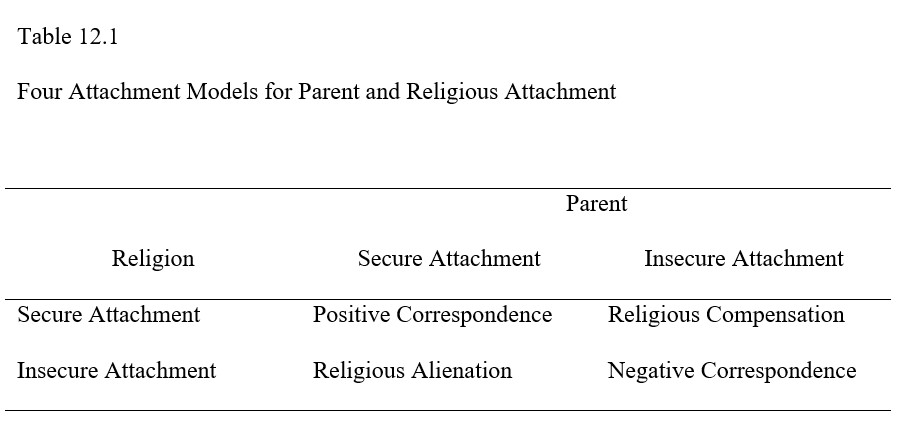
Pargament (1997) expanded upon the compensation hypothesis and showed that the relationship between attachment history and religious beliefs is far from simple. He summarized four relationships between parental and religious attachments extrapolated from Kirkpatrick’s research.  First, if a child had a secure attachment to the parent, he may develop a secure attachment to religion, called ‘ positive correspondence .’  In this scenario, the result of a loving and trusting relationship with one’s parents is transferred to God as well.  This is contrary to the findings of Kirkpatrick and Shaver (1990) which said that securely attached individuals displayed lower levels of religiosity.  More in line with their view is Pargament’s second category, secure attachment to parents and insecure attachment to religion, called ‘ religious alienation .’  Here the person who had a secure attachment to parents may not feel the need to believe in God.  He does not need to compensate for any deficiencies.

The third category is also in line with Kirkpatrick and Shaver’s study.  Modeled after their hypothesis, ‘ religious compensation ’ results from an insecure attachment to parents and a secure attachment to religion.   Finally, an insecure attachment to parents may yield an insecure attachment to religion called ‘ negative correspondence ’ (see Table 12.1).  These insecure parental ties have left the person unequipped to build neither strong adult attachments nor a secure spiritual relationship.  The person may cling to “false gods” like drug and alcohol addiction, food addiction, religious dogmatism, a religious cult, or a codependent relationship.

12.1.3. Health Factors

“ Loneliness kills.” These were the opening words of a March 18, 2015 Time article describing alarming research which shows that loneliness increases the risk of death. How so? According to the meta-analysis of 70 studies published from 1980 to 2014, social isolation increases mortality by 29%, loneliness does so by 26%, and living alone by 32%; but being socially connected leads to higher survival rates (Holt-Lunstad et al., 2015). The authors note, as did Tiwari (2013) earlier, that social isolation and loneliness should be listed as a public health concern as it can lead to poorer health and decreased longevity, as well as CVD (coronary vascular disease; Holt-Lunstad & Smith, 2016). Other ill effects of loneliness include greater stimulated cytokine production due to stress which in turn causes inflammation (Jaremka et al., 2013); greater occurrence of suicidal behavior (Stickley & Koyanagi, 2016); pain, depression, and fatigue (Jarema et al., 2014); and psychotic disorders such as delusional disorders, depressive psychosis, and subjective thought disorder (Badcock et al., 2015).

On a positive note, Stanley, Conwell, Bowen, and Van Orden (2013) found that for older adults who report feeling lonely, owning a pet is one way to feel socially connected. In their study, pet owners were found to be 36% less likely than non-pet owners to report feeling lonely. Those who lived alone and did not own a pet had the greatest odds of reporting loneliness. But the authors offer an admonition – owning a pet, if not managed properly, could actually be deleterious to health. They write, “For example, an older adult may place the well-being of their pet over the safety and health of themselves; they may pay for meals and veterinary services for their pet at the expense of their own meals or healthcare.” Bereavement concerns were also raised, though they say that with careful planning, any negative consequences of owning a pet can be mitigated.

To read the Time article, please visit: http://time.com/3747784/loneliness-mortality/

12.1.4. Social Rejection

Being rejected or ignored by others, called ostracism , hurts. No literally. It hurts. Research by Kross, Berman, Mischel, Smith, and Wager (2011) has shown that when rejected, brain areas such as the secondary somatosensory cortex and dorsal posterior insula which are implicated in the experience of physical pain, become active. So not only are the experiences of physical pain and social rejection distressing, the authors say that they share a common somatosensory representation too.

So, what do you do if you have experienced social rejection? A 2012 article by the American Psychological Association says to seek inclusion elsewhere. Those who have been excluded tend to become more sensitive to opportunities to connect and adjust their behavior as such. They may act more likable, show greater conformity, and comply with the requests of others. Of course, some respond with anger and aggression instead. The article says, “If someone’s primary concern is to reassert a sense of control, he or she may become aggressive as a way to force others to pay attention. Sadly, that can create a downward spiral. When people act aggressively, they’re even less likely to gain social acceptance.” The effects of long-term ostracism can be devastating but non-chronic rejection can be easier to alleviate. Seek out healthy positive connections with both friends and family as a way to combat rejection.

For more on the APA article, see https://www.apa.org/monitor/2012/04/rejection .

• Clarify how proximity affects interpersonal attractiveness.
• Clarify how familiarity affects interpersonal attractiveness.
• Clarify how beauty affects interpersonal attractiveness.
• Clarify how similarity affects interpersonal attractiveness.
• Clarify how reciprocity affects interpersonal attractiveness.
• Clarify how playing hard to get affects interpersonal attractiveness.
• Clarify how intimacy affects interpersonal attractiveness.
• Describe mate selection strategies used by men and women.

On April 7, 2015, Psychology Today published an article entitled, The Four Types of Attraction . Referred to as an attraction pyramid, it places status and health at the bottom, emotional in the middle, and logic at the top of the pyramid. Status takes on two forms. Internal refers to confidence, your skills, and what you believe or your values. External refers to your job, visual markers, and what you own such as a nice car or house. The article states that confidence may be particularly important and overrides external status in the long run. Health can include the way you look, move, smell, and your intelligence. The middle level is emotional which includes what makes us unique, trust and comfort, our emotional intelligence, and how mysterious we appear to a potential suitor. And then at the top is logic which helps us to be sure this individual is aligned with us in terms of life goals such as having kids, getting married, where we will live, etc. The article says – “With greater alignment, there is greater attraction.” Since online romance is trending now, the pyramid flips and we focus on logic, then emotion, and then status and health, but meeting in person is important and should be done as soon as possible. This way, we can be sure there is a physical attraction and can only be validated in person.

To read the article for yourself, visit: https://www.psychologytoday.com/us/blog/valley-girl-brain/201504/the-four-types-attraction

So how accurate is the article? We will tackle several factors on attraction to include proximity, familiarity, physical attractiveness, similarity, reciprocity, the hard-to-get effect, and intimacy, and then close with a discussion of mate selection.

12.2.1. Proximity

First, proximity states that the closer two people live to one another, the more likely they are to interact. The more frequent their interaction, the more likely they will like one another then. Is it possible that individuals living in a housing development would strike up friendships while doing chores? This is exactly what Festinger, Schachter, and Back (1950) found in an investigation of 260 married veterans living in a housing project at MIT. Proximity was the primary factor that led to the formation of friendships. For proximity to work, people must be able to engage in face-to-face communication, which is possible when they share a communication space and time (Monge & Kirste, 1980) and proximity is a determinant of interpersonal attraction for both sexes (Allgeier and Byrne, 1972). A more recent study of 40 couples from Punjab, Pakistan provides cross-cultural evidence of the importance of proximity as well. The authors write, “The results of qualitative analysis showed that friends who stated that they share the same room or same town were shown to have higher scores on interpersonal attraction than friends who lived in distant towns and cities” (pg. 145; Batool & Malik, 2010).

12.2.2. Mere Exposure – A Case for Familiarity?

In fact, the more we are exposed to novel stimuli, the greater our liking of them will be, called the mere exposure effect . Across two studies, Saegert, Swap, & Zajonc (1973) found that the more frequently we are exposed to a stimulus, even if it is negative, the greater our liking of it will be, and that this holds true for inanimate objects but also interpersonal attitudes. They conclude, “…the mere repeated exposure of people is a sufficient condition for enhancement of attraction, despite differences in favorability of context, and in the absence of any obvious rewards or punishments by these people” (pg. 241).

Peskin and Newell (2004) present an interesting study investigating how familiarity affects attraction. In their first experiment, participants rated the attractiveness, distinctiveness, and familiarity of 84 monochrome photographs of unfamiliar female faces obtained from US high school yearbooks. The ratings were made by three different groups – 31 participants for the attractiveness rating, 37 for the distinctiveness rating, and 30 for the familiarity rating – and no participant participated in more than one of the studies. In all three rating studies, a 7-point scale was used whereby 1 indicated that the face was not attractive, distinctive, or familiar and 7 indicated that it was very attractive, distinctive, or familiar. They found a significant negative correlation between attractiveness and distinctiveness and a significant positive correlation between attractiveness and familiarity scores, consistent with the literature.

In the second experiment, 32 participants were exposed to 16 of the 24 most typical and 16 of the 24 most distinctive faces from the experiment and the other 8 faces serving as controls. The controls were shown once during the judgment phase while the 16 typical and 16 distinctive faces were shown six times for a total of 192 trials. Ratings of attractiveness were given during the judgment phase. Results showed that repeated exposure increased attractiveness ratings overall, and there was no difference between typical and distinctive faces. These results were found to be due to increased exposure and not judgment bias or experimental conditions since the attractiveness ratings of the 16 control faces were compared to the same faces from experiment 1 and no significant difference between the two groups was found.

Overall, Peskin and Newell (2004) state that their findings show that increasing the familiarity of faces by increasing exposure led to increased attractiveness ratings. They add, “We also demonstrated that typical faces were found to be more attractive than distinctive faces although both face types were subjected to similar increases in familiarity” (pg. 156).

12.2.3. Physical Attractiveness

Second, we choose who we spend time with based on how attractive they are. Attractive people are seen as more interesting, happier, smarter, sensitive, and moral and as such are liked more than less attractive people. This is partly due to the halo effect or when we hold a favorable attitude to traits that are unrelated. We see beauty as a valuable asset and one that can be exchanged for other things during our social interactions. Between personality, social skills, intelligence, and attractiveness, which characteristic do you think matters most in dating? In a field study randomly pairing subjects at a “Computer Dance” the largest determinant of how much a partner was liked, how much he wanted to date the partner again, and how frequently he asked the partner out, was simply the physical attractiveness of the partner (Walster et al., 1966).

In a more contemporary twist on dating and interpersonal attraction, Luo and Zhang (2009) looked at speed dating. Results showed that the biggest predictor of attraction for both males and females was the physical attractiveness of their partner (reciprocity showed some influence though similarity produced no evidence – both will be discussed shortly so keep it in mind for now).

Is beauty linked to a name though? Garwood et al. (1980) asked 197 college students to choose a beauty queen from six photographs, all equivalent in terms of physical attractiveness. Half of the women in the photographs had a desirable first name while the other half did not. Results showed that girls with a desirable first name received 158 votes while those with an undesirable first name received just 39 votes.

So why beauty? Humans display what is called a beauty bias . Struckman-Johnson and Struckman- Johnson (1994) investigated the reaction of 277 male, middle-class, Caucasian college students to a vignette in which they were asked to imagine receiving an uninvited sexual advance from a casual female acquaintance. The vignette displayed different degrees of coercion such as low-touch, moderate-push, high-threat, and very high-weapon. The results showed that men had a more positive reaction to the sexual advance of a female acquaintance who was attractive and who used low or moderate levels of coercion than to an unattractive female.

What about attractiveness in the workplace? Hosoda, Stone-Romero, and Coats (2006) found considerable support for the notion that attractive individuals fare better in employment-related decisions (i.e., hiring and promotions) than unattractive individuals. Although there is a beauty bias, the authors found that its strength has weakened over the past few decades.

12.2.4. Similarity

You have likely heard the expressions “Opposites attract” and “Birds of a feather flock together.” The former expression contradicts the latter, and so this leads us to wonder which is it? Research shows that we are most attracted to people who are like us in terms of our religious and political beliefs, values, appearance, educational background, age, and other demographic variables (Warren, 1966). Thus, we tend to choose people who are similar to us in attitudes and interests as this leads to a more positive evaluation of them. Their agreement with our choices and beliefs helps to reduce any uncertainty we face regarding social situations and improves our understanding of the situation. You might say their similarity also validates our own values, beliefs, and attitudes as they have arrived at the same conclusions that we have. This occurs with identification with sports teams. Our perceived similarity with the group leads to group-derived self-definition more so than the attractiveness of the group such that, “… a team that is “crude, rude, and unattractive” may be appealing to fans who have the same qualities, but repulsive to fans who are more “civilized”.” The authors suggest that sports marketers could emphasize the similarities between fans and their teams (Fisher, 1998). Another form of similarity is in terms of physical attractiveness. According to the matching hypothesis , we date others who are similar to us in terms of how attractive they are (Feingold, 1988; Huston, 1973; Bersheid et al., 1971; Walster, 1970).

12.2.5. Reciprocity

Fourth, we choose people who are likely to engage in a mutual exchange with us. We prefer people who make us feel rewarded and appreciated and in the spirit of reciprocation, we need to give something back to them. This exchange continues so long as both parties regard their interactions to be mutually beneficial or the benefits of the exchange outweigh the costs (Homans, 1961; Thibaut & Kelley, 1959). If you were told that a stranger you interacted with liked you, research shows that you would express a greater liking for that person as well (Aronson & Worchel, 1966) and the same goes for reciprocal desire (Greitmeyer, 2010).

12.2.6. Playing Hard to Get

Does playing hard to get make a woman (or man) more desirable than the one who seems eager for an alliance? Results of five experiments said that it does not though a sixth experiment suggests that if the woman is easy for a particular man to get but hard for all other men to get, she would be preferred over a woman who is uniformly hard or easy to get, or is a woman for which the man has no information about. Men gave these selective women all of the assets (i.e. selective, popular, friendly, warm, and easy going) but none of the liabilities (i.e. problems expected in dating) of the uniformly hard to get and easy to get women. The authors state, “It appears that a woman can intensify her desirability if she acquires a reputation for being hard-to-get and then, by her behavior, makes it clear to a selected romantic partner that she is attracted to him” (pg. 120; Walster et al., 1973). Dai, Dong, and Jia (2014) predicted and found that when person B plays hard to get with person A, this will increase A’s wanting of B but simultaneously decrease A’s liking of B, only if A is psychologically committed to pursuing further relations with B. Otherwise, the hard to get strategy will result in decreased wanting and liking.

12.2.7. Intimacy

Finally, intimacy occurs when we feel close to and trust in another person. This factor is based on the idea of self-disclosure or telling another person about our deepest held secrets, experiences, and beliefs that we do not usually share with others. But this revealing of information comes with the expectation of a mutual self-disclosure from our friend or significant other. We might think that self-disclosure is difficult online but a study of 243 Facebook users shows that we tell our personal secrets on Facebook to those we like and that we feel we can disclose such personal details to people with whom we talk often and come to trust (Sheldon, 2009).

This said, there is a possibility we can overshare, called overdisclosure , which may lead to a reduction in our attractiveness. What if you showed up for class a few minutes early and sat next to one of your classmates who proceeded to give you every detail of their weekend of illicit drug use and sexual activity? This would likely make you feel uncomfortable and seek to move to another seat.

12.2.8. Mate Selection

As you will see in a bit, men and women have vastly different strategies when it comes to selecting a mate. This leads us to ask why, and the answer is rooted in evolutionary psychology. Mate selection occurs universally in all human cultures. In a trend seen around the world, Buss (2004) said that since men can father a nearly unlimited number of children, they favor signs of fertility in women to include being young, attractive, and healthy. Since they also want to know that the child is their own, they favor women who will be sexually faithful to them.

In contrast, women favor a more selective strategy given the incredible time investment having a child involves and the fact that she can only have a limited number of children during her life. She looks for a man who is financially stable and can provide for her children, typically being an older man. In support of the difference in age of a sexual partner pursued by men and women, Buss (1989) found that men wanted to marry women 2.7 years younger while women preferred men 3.4 years older. Also, this finding emerged cross-culturally.

• Describe how the social exchange theory explains relationships.
• Describe how the equity theory explains relationships.
• List and describe types of relationships.
• Define love and describe its three components according to Sternberg.
• Define jealousy.

12.3.1. Social Exchange Theory

Recall from Section 11.2.9 that social exchange theory is the idea that we utilize a minimax strategy whereby we seek to maximize our rewards all while minimizing our costs. In terms of relationships, those that have less costs and more rewards will be favored, last longer, and be more fulfilling. Rewards include having someone to console us during difficult times, companionship, the experience of love, and having a committed sexual partner for romantic relationships. Costs include the experience of conflict, having to compromise, and needing to sacrifice for another.

12.3.2. Equity Theory

Equity theory (Walster et al., 1978) consists of four propositions. First, it states that individuals will try to maximize outcomes such that rewards win out over punishments. Second, groups will evolve systems for equitably apportioning rewards and punishments among members and members will be expected to adhere to these systems. Those who are equitable to others will be rewarded while those who are not will be punished. Third, individuals in inequitable relationships will experience distress proportional to the inequity. Fourth, those in inequitable relationships will seek to eliminate their distress by restoring equity and will work harder to achieve this the greater the distress they experience. The goal is for all participants to feel they are receiving equal relative gains from the relationship.

According to Hatfield and Traupmann (1981) if an individual feels that the ratio between benefits and costs are disproportionately in favor of the other partner, he or she may feel ripped off or underbenefited, and experience distress. So, what can be done about this? The authors state, “There are only two ways that people can set things right: they can re-establish actual equity or psychological equity. In the first case they can inaugurate real changes in their relationships, e.g. the underbenefited may well ask for more out of their relationships, or their overbenefited partners may offer to try to give more. In the latter case couples may find it harder to change their behavior than to change their minds and so prefer to close their eyes and to reassure themselves that “really, everything is in perfect order”” (pg.168).

12.3.3. Types of Relationships

Relationships can take on a few different forms. In what are called communal relationships, there is an expectation of mutual responsiveness from each member as it relates to tending to member’s needs while exchange relationships involve the expectation of reciprocity in a form of tit-for-tat strategy. This leads to what are called intimate or romantic relationships in which you feel a very strong sense of attraction to another person in terms of their personality and physical features. Love is often a central feature of intimate relationships.

12.3.4. Love

One outcome of this attraction to others, or the need to affiliate/belong is love. What is love? According to a 2011 article in Psychology Today entitled ‘ What is Love, and What Isn’t It? ’ love is a force of nature, is bigger than we are, inherently free, cannot be turned on as a reward or off as a punishment, cannot be bought, cannot be sold, and cares what becomes of us). Adrian Catron writes in an article entitled, “What is Love? A Philosophy of Life” that “the word love is used as an expression of affection towards someone else….and expresses a human virtue that is based on compassion, affection and kindness.” He goes on to say that love is a practice and you can practice it for the rest of your life. ( https://www.huffpost.com/entry/what-is-love-a-philosophy_b_5697322 ). And finally, the Merriam Webster dictionary online defines love as “strong affection for another arising out of kinship or personal ties” and “attraction based on sexual desire: affection and tenderness felt by lovers.” (Source: https://www.merriam-webster.com/dictionary/love ).

Robert Sternberg (1986) said love is composed of three main parts (called the triangular theory of love ): intimacy, commitment, and passion. First, intimacy is the emotional component and involves how much we like, feel close to, and are connected to another person. It grows steadily at first, slows down, and then levels off. Features include holding the person in high regard, sharing personal affect with them, and giving them emotional support in times of need. Second, commitment is the cognitive component and occurs when you decide you truly love the person. You decide to make a long-term commitment to them and as you might expect, is almost non-existent when a relationship begins and is the last to develop usually. If a relationship fails, commitment would show a pattern of declining over time and eventually returns to zero. Third, passion represents the motivational component of love and is the first of the three to develop. It involves attraction, romance, and sex and if a relationship ends, passion can fall to negative levels as the person copes with the loss.

This results in eight subtypes of love which explains differences in the types of love we express. For instance, the love we feel for our significant other will be different than the love we feel for a neighbor or coworker, and reflect different aspects of the components of intimacy, commitment, and passion as follows:

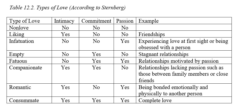
12.3.4.1. Jealousy. The dark side of love is what is called jealousy , or a negative emotional state arising due to a perceived threat to one’s relationship. Take note of the word perceived here. The threat does not have to be real for jealousy to rear its ugly head and what causes men and women to feel jealous varies. For women, a man’s emotional infidelity leads her to fear him leaving and withdrawing his financial support for her offspring, while sexual infidelity is of greater concern to men as he may worry that the children he is supporting are not his own. Jealousy can also arise among siblings who are competing for their parent’s attention, among competitive coworkers especially if a highly desired position is needing to be filled, and among friends. From an evolutionary perspective, jealousy is essential as it helps to preserve social bonds and motivates action to keep important relationships stable and safe. But it can also lead to aggression (Dittman, 2005) and mental health issues.

• Describe Gottman’s Four Horsemen of the Apocalypse.
• Propose antidotes to the horsemen.
• Clarify the importance of forgiveness in relationships.

12.4.1. Communication, Conflict, and Successful Resolution

John Gottman used the metaphor of the Four Horsemen of the Apocalypse from the New Testament to describe communication styles that can predict the end of a relationship. Though not conquest, war, hunger, and death, Gottman instead used the terms criticism, contempt, defensiveness, and stonewalling. Each will be discussed below, as described on Gottman’s website: https://www.gottman.com/blog/the-four-horsemen-recognizing-criticism-contempt-defensiveness-and-stonewalling/

First, criticism occurs when a person attacks their partner at their core character “or dismantling their whole being” when criticized. An example might be calling them selfish and saying they never think of you. It differs from a complaint which typically involves a specific issue. For instance, one night in March 2019 my wife was stuck at work until after 8pm. I was upset as she did not call to let me know what was going on and we have an agreement to inform one another about changing work schedules. Criticism can become pervasive and when it does, it leads to the other, far deadlier horsemen. “It makes the victim feel assaulted, rejected, and hurt, and often causes the perpetrator and victim to fall into an escalating pattern where the first horseman reappears with greater and greater frequency and intensity, which eventually leads to contempt.”

The second horseman is contempt which involves treating others with disrespect, mocking them, ridiculing, being sarcastic, calling names, or mimicking them. The point is to make the target feel despised and worthless. “Most importantly, contempt is the single greatest predictor of divorce . It must be eliminated.”

Defensiveness is the third horseman and is a response to criticism. When we feel unjustly accused, we have a tendency to make excuses and play the innocent victim to get our partner to back off. Does it work though? “Although it is perfectly understandable to defend yourself if you’re stressed out and feeling attacked, this approach will not have the desired effect. Defensiveness will only escalate the conflict if the critical spouse does not back down or apologize. This is because defensiveness is really a way of blaming your partner, and it won’t allow for healthy conflict management.”

Stonewalling is the fourth horseman and occurs when the listener withdraws from the interaction, shuts down, or stops responding to their partner. They may tune out, act busy, engage in distracting behavior, or turn away and stonewalling is a response to contempt. “It is a result of feeling physiologically flooded, and when we stonewall, we may not even be in a physiological state where we can discuss things rationally.”

Conflict is an unavoidable reality of relationships. The good news is that each horseman has an antidote to stop it. How so?

• To combat criticism, engage in gentle start up . Talk about your feelings using “I” statements and not “you” and express what you need to in a positive way. As the website demonstrates, instead of saying “You always talk about yourself. Why are you always so selfish?” say, “I’m feeling left out of our talk tonight and I need to vent. Can we please talk about my day?”
• To combat contempt, build a culture of appreciation and respect . Regularly express appreciation, gratitude, affection, and respect for your partner. The more positive you are, the less likely that contempt will be expressed. Instead of saying, “You forgot to load the dishwasher again? Ugh. You are so incredibly lazy.” (Rolls eyes.) say, “I understand that you’ve been busy lately, but could you please remember to load the dishwasher when I work late? I’d appreciate it.”
• To combat defensiveness, take responsibility . You can do this for just part of the conflict. A defensive comment might be, “It’s not my fault that we’re going to be late. It’s your fault since you always get dressed at the last second.” Instead, say, “I don’t like being late, but you’re right. We don’t always have to leave so early. I can be a little more flexible.”
• To combat stonewalling, engage in physiological self-soothing . Arguing increases one’s heart rate, releases stress hormones, and activates our flight-fight response. By taking a short break, we can calm down and “return to the discussion in a respectful and rational way.” Failing to take a break could lead to stonewalling and bottling up emotions, or exploding like a volcano at your partner, or both. “So, when you take a break, it should last at least twenty minutes because it will take that long before your body physiologically calms down. It’s crucial that during this time you avoid thoughts of righteous indignation (“I don’t have to take this anymore”) and innocent victimhood (“Why is he always picking on me?”). Spend your time doing something soothing and distracting, like listening to music, reading, or exercising. It doesn’t really matter what you do, as long as it helps you to calm down.”

12.4.2. Forgiveness

According to the Mayo Clinic, forgiveness involves letting go of resentment and any thought we might have about getting revenge on someone for past wrongdoing. So what are the benefits of forgiving others? Our mental health will be better, we will experience less anxiety and stress, we may experience fewer symptoms of depression, our heart will be healthier, we will feel less hostility, and our relationships overall will be healthier.

It’s easy to hold a grudge. Let’s face it, whatever the cause, it likely left us feeling angry, confused, and sad. We may even be bitter not only to the person who slighted us but extend this to others who had nothing to do with the situation. We might have trouble focusing on the present as we dwell on the past and feel like life lacks meaning and purpose.

But even if we are the type of person who holds grudges, we can learn to forgive. The Mayo Clinic offers some useful steps to help us get there. First, we should recognize the value of forgiveness. Next, we should determine what needs healing and who we should forgive and for what. Then we should consider joining a support group or talk with a counselor. Fourth, we need to acknowledge our emotions, the harm they do to us, and how they affect our behavior. We then attempt to release them. Fifth, choose to forgive the person who offended us leading to the final step of moving away from seeing ourselves as the victim and “release the control and power the offending person and situation have had in your life.”

At times, we still cannot forgive the person. They recommend practicing empathy so that we can see the situation from their perspective, praying, reflecting on instances of when you offended another person and they forgave you, and be aware that forgiveness does not happen all at once but is a process.

Read the article by visiting: https://www.mayoclinic.org/healthy-lifestyle/adult-health/in-depth/forgiveness/art-20047692

Module Recap

That’s it. With the close of this module, we also finish the book. We hope you enjoyed learning about attraction and the various factors on it, types of relationships, and complications we might endure. As we learned, conflict is inevitable in any type of relationship, but there is hope. Never give up or give in.

Module 12 is the last in Part IV: How We Relate to Others.

2nd edition

Share This Book

• Increase Font Size

Thank you for visiting nature.com. You are using a browser version with limited support for CSS. To obtain the best experience, we recommend you use a more up to date browser (or turn off compatibility mode in Internet Explorer). In the meantime, to ensure continued support, we are displaying the site without styles and JavaScript.

• View all journals
• Explore content
• About the journal
• Publish with us
• Sign up for alerts
• Published: 01 September 2001

Neurophysiological mechanisms underlying the understanding and imitation of action

• Giacomo Rizzolatti 1 , 2 ,
• Leonardo Fogassi 1 &
• Vittorio Gallese 1  

Nature Reviews Neuroscience volume  2 ,  pages 661–670 ( 2001 ) Cite this article

12k Accesses

2141 Citations

92 Altmetric

Metrics details

What are the neural bases of action understanding? Although this capacity could merely involve visual analysis of the action, it has been argued that we actually map this visual information onto its motor representation in our nervous system. Here we discuss evidence for the existence of a system, the 'mirror system', that seems to serve this mapping function in primates and humans, and explore its implications for the understanding and imitation of action.

This is a preview of subscription content, access via your institution

Access options

Subscribe to this journal

Receive 12 print issues and online access

176,64 € per year

only 14,72 € per issue

Buy this article

• Purchase on Springer Link
• Instant access to full article PDF

Prices may be subject to local taxes which are calculated during checkout

Similar content being viewed by others

Delineating visual, auditory and motor regions in the human brain with functional neuroimaging: a BrainMap-based meta-analytic synthesis

Action execution and action observation elicit mirror responses with the same temporal profile in human SII

Activity in primate visual cortex is minimally driven by spontaneous movements

Gross, C. G., Rocha-Miranda, C. E. & Bender, D. B. Visual properties of neurons in the inferotemporal cortex of the macaque. J. Neurophysiol. 35 , 96–111 (1972).

Article   CAS   PubMed   Google Scholar  

Tanaka, K., Saito, H. A., Fukada, Y. & Moriya, M. Coding visual images of objects in the inferotemporal cortex of the macaque monkey. J. Neurophysiol. 66 , 170–189 (1991).

Ungerleider, L. G. & Haxby, I. V. “What” and “where” in the human brain. Curr. Opin. Neurobiol. 4 , 157–165 (1994).

Carey, D. P., Perrett, D. I. & Oram, M. W. in Handbook of Neuropsychology: Action and Cognition Vol. 11 (eds Jeannerod, M. & Grafman, J.) 111–130 (Elsevier, Amsterdam, 1997).

Google Scholar  

Logothetis, N. Object vision and visual awareness. Curr. Opin. Neurobiol. 8 , 536–544 (1998).

Allison, T., Puce, A. & McCarthy, G. Social perception from visual cues: role of the STS region. Trends Cogn. Sci. 4 , 267–278 (2000).

Kanwisher, N. Domain specificity in face perception. Nature Neurosci. 3 , 759–763 (2000).

Merleau-Ponty, M. Phenomenology of Perception (Routledge, London, 1962).

Gallese, V. The “shared manifold” hypothesis: from mirror neurons to empathy. J. Conscious Stud. 8 , 33–50 (2001).

Gallese, V., Fadiga, L., Fogassi, L. & Rizzolatti, G. Action recognition in the premotor cortex. Brain 119 , 593–609 (1996).

Article   PubMed   Google Scholar  

Rizzolatti, G., Fadiga, L., Fogassi, L. & Gallese, V. Premotor cortex and the recognition of motor actions. Brain Res. Cogn. Brain Res. 3 , 131–141 (1996).

Rizzolatti, G. et al. Functional organization of inferior area 6 in the macaque monkey: II. Area F5 and the control of distal movements. Exp. Brain Res. 71 , 491–507 (1988).

Murata, A. et al. Object representation in the ventral premotor cortex (area F5) of the monkey. J. Neurophysiol. 78 , 2226–2230 (1997).

Rizzolatti G., Fogassi, L. & Gallese, V. in The Cognitive Neurosciences 2nd edn (ed. Gazzaniga, M. S.) 539–552 (MIT Press, Cambridge, Massachusetts, 2000).

Perrett, D. I. et al. Frameworks of analysis for the neural representation of animate objects and actions. J. Exp. Biol. 146 , 87–113 (1989).

CAS   PubMed   Google Scholar  

Perrett, D. I., Mistlin, A. J., Harries, M. H. & Chitty, A. J. in Vision and Action: The Control of Grasping (ed. Goodale, M. A.) 163–342 (Ablex, Norwood, New Jersey, 1990).

Jellema, T. & Perrett, D. I. in Attention & Performance XIX. Common Mechanisms in Perception and Action (eds Prinz, W. & Hommel, B.) (Oxford Univ. Press, Oxford, in the press).

Petrides, M. & Pandya, D. N. Projections to the frontal cortex from the posterior parietal region in the rhesus monkey. J. Comp. Neurol. 228 , 105–116 (1984).

Matelli, M., Camarda, R., Glickstein, M. & Rizzolatti, G. Afferent and efferent projections of the inferior area 6 in the macaque monkey. J. Comp. Neurol. 251 , 281–298 (1986).

Cavada, C. & Goldman-Rakic, P. S. Posterior parietal cortex in rhesus monkey: II. Evidence for segregated corticocortical networks linking sensory and limbic areas with the frontal lobe. J. Comp. Neurol. 287 , 422–445 (1989).

Seltzer, B. & Pandya, D. N. Parietal, temporal, and occipital projections to cortex of the superior temporal sulcus in the rhesus monkey: a retrograde tracer study. J. Comp. Neurol. 15 , 445–463 (1994).

Article   Google Scholar  

Rizzolatti, G., Luppino, G. & Matelli, M. The organization of the cortical motor system: new concepts. Electroencephalogr. Clin. Neurophysiol. 106 , 283–296 (1998).

Fogassi, L., Gallese, V., Fadiga, L. & Rizzolatti, G. Neurons responding to the sight of goal directed hand/arm actions in the parietal area PF (7b) of the macaque monkey. Soc. Neurosci. Abstr. 24 , 257 (1998).

Gallese, V., Fogassi, L., Fadiga, L. & Rizzolatti, G. in Attention & Performance XIX. Common Mechanisms in Perception and Action (eds Prinz, W. & Hommel, B.) 334–355 (Oxford Univ. Press, Oxford, in the press).

Amaral, D. G. et al. in The Amygdala: Neurobiological Aspects of Emotion, Memory, and Mental Disfunction (ed. Aggleton, J. P.) 1–66 (Wiley-Liss, New York, 1992).

Baron-Cohen, S. Mindblindness: an Essay on Autism and Theory of Mind (MIT Press/Bradford Books, 1995).

Adolphs, R. Social cognition and the human brain. Trends Cogn. Sci. 3 , 469–479 (1999).

Brothers, L., Ring, B. & Kling, A. Response of neurons in the macaque amygdala to complex social stimuli. Behav. Brain Res. 41 , 199–213 (1990).

Brothers, L. & Ring, B. A neuroethological framework for the representation of minds. J. Cogn. Neurosci. 4 , 107–118 (1992).

Bonda, E., Petrides, M., Ostry, D. & Evans, A. Specific involvement of human parietal systems and the amygdala in the perception of biological motion. J. Neurosci. 16 , 3737–3744 (1996).

Article   CAS   PubMed   PubMed Central   Google Scholar  

Carr, L., Iacoboni, M., Dubeau, M.-C., Mazziotta, J. C. & Lenzi, G. L. Observing and imitating emotion: implications for the neurological correlates of empathy. Proc. First Int. Conf. Soc. Cogn. Neurosci. (2001).

Cole, J. D. About Face (MIT Press, Cambridge, Massachusetts, 1999).

Cole, J. D. Empathy needs a face. J. Conscious Stud. 8 , 51–68 (2001).

Rizzolatti, G., Fadiga, L., Fogassi, L. & Gallese, V. Resonance behaviors and mirror neurons. Arch. Ital. Biol. 137 , 85–100 (1999).

Gastaut, H. J. & Bert, J. EEG changes during cinematographic presentation. Electroencephalogr. Clin. Neurophysiol. 6 , 433–444 (1954).

Cohen-Seat, G., Gastaut, H., Faure, J. & Heuyer, G. Etudes expérimentales de l'activité nerveuse pendant la projection cinématographique. Rev. Int. Filmol. 5 , 7–64 (1954).

Chatrian, G. E. in Handbook of Electroencephalography (ed. Remond, A.) 104–114 (Elsevier, Amsterdam, 1976).

Cochin, S., Barthelemy, C., Lejeune, B., Roux, S., & Martineau, J. Perception of motion and qEEG activity in human adults. Electroencephalogr. Clin. Neurophysiol. 107 , 287–295 (1998).

Cochin, S., Barthelemy, C., Roux, S. & Martineau, J. Observation and execution of movement: similarities demonstrated by quantified electroencephalograpy. Eur. J. Neurosci. 11 , 1839–1842 (1999).

Altschuler, E. L., Vankov, A., Wang, V., Ramachandran, V. S. & Pineda, J. A. Person see, person do: human cortical electrophysiological correlates of monkey see monkey do cell. Soc. Neurosci. Abstr. 23 , 719 (1997).

Altschuler, E. L. et al. Mu wave blocking by observation of movement and its possible use as a tool to study theory of other minds. Soc. Neurosci. Abstr. 26 , 68 (2000).

Salmelin, R. & Hari, R. Spatiotemporal characteristics of sensorimotor neuromagnetic rhythms related to thumb movement. Neuroscience 60 , 537–550 (1994).

Hari, R. & Salmelin, R. Human cortical oscillations: a neuromagnetic view through the skull. Trends Neurosci. 20 , 44–49 (1997).

Salenius, S., Schnitzler, A., Salmelin, R., Jousmaki, V. & Hari, R. Modulation of human cortical rolandic rhythms during natural sensorimotor tasks. Neuroimage 5 , 221–228 (1997).

Hari, R. et al. Activation of human primary motor cortex during action observation: a neuromagnetic study. Proc. Natl Acad. Sci. USA 95 , 15061–15065 (1998).

Fadiga, L. Fogassi, L., Pavesi, G. & Rizzolatti, G. Motor facilitation during action observation: a magnetic stimulation study. J. Neurophysiol. 73 , 2608–2611 (1995).

Strafella, A. P. & Paus, T. Modulation of cortical excitability during action observation: a transcranial magnetic stimulation study. Neuroreport 11 , 2289–2292 (2000).

Baldissera, F., Cavallari, P., Craighero, L. & Fadiga, L. Modulation of spinal excitability during observation of hand actions in humans. Eur. J. Neurosci. 13 , 190–194 (2001).

Rizzolatti, G. et al. Localization of grasp representation in humans by PET: 1. Observation versus execution. Exp. Brain Res. 111 , 246–252 (1996).

Grafton, S. T., Arbib, M. A., Fadiga, L. & Rizzolatti, G. Localization of grasp representations in humans by PET: 2. Observation compared with imagination. Exp. Brain Res. 112 , 103–111 (1996).

Decety, J. et al. Brain activity during observation of actions. Influence of action content and subject's strategy. Brain 120 , 1763–1777 (1997).

Grèzes, J., Costes, N. & Decety, J. Top–down effect of strategy on the perception of human biological motion: a PET investigation. Cogn. Neuropsychol. 15 , 553–582 (1998).

Rizzolatti, G. & Arbib, M. A. Language within our grasp. Trends Neurosci. 21 , 188–194 (1998).

Von Bonin, G. & Bailey, P. The Neocortex of Macaca Mulatta (Univ. Illinois Press, Urbana, 1947).

Petrides, M. & Pandya, D. N. in Handbook of Neuropsychology Vol. IX (eds Boller, F. & Grafman, J.) 17–58 (Elsevier, New York, 1997).

Krams, M., Rushworth, M. F., Deiber, M. P., Frackowiak, R. S. & Passingham, R. E. The preparation, execution and suppression of copied movements in the human brain. Exp. Brain Res. 120 , 386–398 (1998).

Binkofski, F. et al. A fronto-parietal circuit for object manipulation in man: evidence from an fMRI study. Eur. J. Neurosci. 11 , 3276–3286 (1999).

Ehrsson, H. H. et al. Cortical activity in precision- versus power-grip tasks: an fMRI study. J. Neurophysiol. 83 , 528–536 (2000).

Iacoboni, M. et al. Cortical mechanisms of human imitation. Science 286 , 2526–2528 (1999).

Nishitani, N. & Hari, R. Temporal dynamics of cortical representation for action. Proc. Natl Acad. Sci. USA 97 , 913–918 (2000).

Buccino, G. et al. Action observation activates premotor and parietal areas in a somatotopic manner: an fMRI study. Eur. J. Neurosci. 13 , 400–404 (2001).

Jellema, T., Baker, C. I., Wicker, B. & Perrett, D. I. Neural representation for the perception of the intentionality of actions. Brain Cogn 44 , 280–302 (2000).

Umiltà, M. A. et al. “I know what you are doing”: a neurophysiological study. Neuron 32 , 91–101 (2001).

Assad, J. A. & Maunsell, J. H. R. Neuronal correlates of inferred motion in primates posterior parietal cortex. Nature 373 , 518–521 (1995).

Fillion, C. M., Washburn, D. A. & Gulledge, J. P. Can monkeys ( Macaca mulatta ) represent invisible displacement? J. Comp. Psychol. 110 , 386–395 (1996).

Visalberghi, E. & Fragaszy, D. in “Language” and Intelligence in Monkeys and Apes (eds Parker, S. T. & Gibson, K. R.) 247–273 (Cambridge Univ. Press, Cambridge, Massachusetts, 1990).

Book   Google Scholar  

Visalberghi, E. & Fragaszy, D. in Imitation in Animals and Artifacts (eds Dautenhahn, K. & Nehaniv, C.) (MIT Press, Boston, Massachusetts, in the press).

Rizzolatti, G., Fadiga, L., Fogassi, L. & Gallese, V. in The Imitative Mind: Development, Evolution and Brain Bases (eds Prinz, W. & Meltzoff, A.) (Cambridge Univ. Press, Cambridge, in the press).

Spence, K. W. Experimental studies of learning and higher mental processes in infra-human primates. Psychol. Bull. 34 , 806–850 (1937).

Thorpe, W. H. Learning and Instinct in Animals 2nd edn (Methuen and Co. Ltd, London, 1963).

Whiten, A. & Ham, R. On the nature and evolution of imitation in the animal kingdom: reappraisal of a century of research. Adv. Study Behav. 21 , 239–283 (1992).

Whiten, A. Imitation of the sequential structure of actions by chimpanzees (Pan troglodytes). J. Comp. Psychol. 112 , 270–281 (1998).

Tomasello, M. & Call, J. Primate Cognition (Oxford Univ. Press, Oxford, 1997).

Byrne, R. W. The Thinking Ape. Evolutionary Origins of Intelligence (Oxford Univ. Press, Oxford, 1995).

Tinbergen, N. The Herring Gull's World (Collins, London, 1953).

Meltzoff, A. N. & Moore, M. K. Imitation of facial and manual gestures by human neonates. Science 198 , 75–78 (1977).

Bråten, S. (ed.) Intersubjective Communication and Emotion in Early Ontogeny (Cambridge Univ. Press, Cambridge, 1999).

Darwin, C. The Expression of the Emotions in Man and Animals (J. Murray, London, 1872).

Dimberg, U., Thunberg, M. & Elmehed, K. Unconscious facial reactions to emotional facial expressions. Psychol. Sci. 11 , 86–89 (2000).

Hepp-Reymond, M. C., Hüsler, E. J., Maier, M. A. & Qi, H.-X. Force-related neuronal activity in two regions of the primate ventral premotor cortex. Can. J. Physiol. Pharmacol. 72 , 571–579 (1994).

Fogassi, L. et al. Visual responses in the dorsal premotor area F2 of the macaque monkey. Exp. Brain Res. 128 , 194–199 (1999).

Gentilucci, M. et al. Functional organization of inferior area 6 in the macaque monkey. I. Somatotopy and the control of proximal movements. Exp. Brain Res. 71 , 475–490 (1988).

Hoshi, E. & Tanji, J. Integration of target and body-part information in the premotor cortex when planning action. Nature 408 , 466–470 (2000).

Byrne, R. Imitation in action. Adv. Study Behav. (in the press).

Byrne, R. W. Imitation without intentionality: using string-parsing to copy the organization of behaviour. Anim. Cogn 2 , 63–72 (1999).

Hikosaka, O., Rand, M. K., Miyachi, S. & Miyashita, K. Learning of sequential movements in the monkey: process of learning and retention of memory. J. Neurophysiol. 74 , 1652–1661 (1995).

Hikosaka, O., Miyashita, K., Miyachi, S., Sakai, K. & Lu, X. Differential roles of the frontal cortex, basal ganglia, and cerebellum in visuomotor sequence learning. Neurobiol. Learn. Mem. 70 , 137–149 (1998).

Hikosaka, O. et al. in The Cognitive Neurosciences 2nd edn (ed. Gazzaniga, M. S.) 553–572 (MIT Press, Cambridge, Massachusetts, 2000).

Tanji, J. New concepts of the supplementary motor area. Curr. Opin. Neurobiol. 6 , 782–787 (1996).

Tanji, J., Shima, K. & Mushiake, H. Multiple cortical motor areas and temporal sequencing of movements. Brain Res. Cogn. Brain Res. 5 , 117–122 (1996).

Shima, K. & Tanji, J. Neuronal activity in the supplementary and presupplementary motor areas for temporal organization of multiple movements. J. Neurophysiol. 84 , 2148–2160 (2000).

Wolpert, D. M. Computational approaches to motor control. Trends Cogn. Sci. 1 , 209–216 (1997).

Wolpert, D. M., Ghahramani, Z. & Jordan, M. I. An internal model for sensorimotor integration. Science 269 , 1880–1882 (1995).

Kawato, M. Internal models for motor control and trajectory planning. Neuroreport 9 , 718–727 (1999).

CAS   Google Scholar  

Arbib, M. E. & Rizzolatti, G. in The Nature of Concepts. Evolution, Structure, and Representation (ed. Van Loocke, P.) 128–154 (Routledge, London, 1999).

Greenwald, A. G. Sensory feedback mechanisms in performance control: with special reference to the ideo-motor mechanism. Psychol. Rev. 77 , 73–99 (1970).

Prinz, W. Perception and action planning. Eur. J. Cogn. Psychol. 9 , 129–154 (1997).

Brass, M., Bekkering, H., Wohlschlager, A. & Prinz, W. Compatibility between observed and executed finger movements: comparing symbolic, spatial and imitative cues. Brain Cogn 44 , 124–143 (2000).

Iacoboni, M. et al. Mirror properties in a sulcus angularis area. Neuroimage 5 , S821 (2000).

Gallese, V. & Goldman, A. Mirror neurons and the simulation theory of mind-reading. Trends Cogn. Sci. 12 , 493–501 (1998).

Frith, C. D. & Frith, U. Interacting minds: a biological basis. Science 286 , 1692–1695 (1999).

Blakemore, S.-J. & Decety, J. From the perception of action to the understanding of intention. Nature Rev. Neurosci. 2 , 561–567 (2001).

Article   CAS   Google Scholar  

Williams, J. H. G., Whiten, A., Suddendorf, T. & Perrett, D. I. Imitation, mirror neurons, and autism. Neurosci. Biobehav. Rev. 25 , 287–295 (2001).

Von Economo, C. The Cytoarchitectonics of the Human Cerebral Cortex (Oxford Univ. Press, London, 1929).

Download references

Author information

Authors and affiliations.

the Istituto di Fisiologia Umana, Università di Parma, Via Volturno 39, Parma, I-43100, Italy

Giacomo Rizzolatti, Leonardo Fogassi & Vittorio Gallese

Giacomo Rizzolatti

You can also search for this author in PubMed   Google Scholar

Related links

Mit encyclopedia of cognitive sciences.

Positron emission tomography

Motor control

Magnetic resonance imaging

Attribution theory

Perception of motion

Theory of mind

A variant of the transcranial magnetic stimulation technique, in which two coils are used to generate magnetic fields in quick succession over the same cortical region or in different regions at the same time.

Also known as the Hoffmann reflex, the H reflex results from the stimulation of sensory fibres, which causes an excitatory potential in the motor neuron pool after a synaptic delay. Exceeding the potential threshold for a given motor neuron generates an action potential. The resulting discharge will cause the muscle fibres innervated by that neurone to be activated.

A movement not directed towards an object.

A disorder characterized by facial paralysis, attributed to defects in the development of the sixth (abducens) and seventh (facial) cranial nerves.

A philosophical movement founded by the German Edward Husserl, dedicated to describing the structures of experience as they present themselves to consciousness, without recourse to theory, deduction or assumptions from other disciplines, such as the natural sciences.

Stimuli devised by the Swedish psychologist Johannson to study biological motion without interference from shape. Light sources are attached to the joints of people and their movements are recorded in a dark environment.

A technique used to stimulate relatively restricted areas of the human cerebral cortex. It is based on the generation of a strong magnetic field near the area of interest which, if changed rapidly enough, will induce an electric field sufficient to stimulate neurons.

Rights and permissions

Reprints and permissions

About this article

Cite this article.

Rizzolatti, G., Fogassi, L. & Gallese, V. Neurophysiological mechanisms underlying the understanding and imitation of action. Nat Rev Neurosci 2 , 661–670 (2001). https://doi.org/10.1038/35090060

Download citation

Issue Date : 01 September 2001

DOI : https://doi.org/10.1038/35090060

Share this article

Anyone you share the following link with will be able to read this content:

Sorry, a shareable link is not currently available for this article.

Provided by the Springer Nature SharedIt content-sharing initiative

This article is cited by

Ultra-high field fmri identifies an action-observation network in the common marmoset.

• Alessandro Zanini
• Audrey Dureux
• Stefan Everling

Communications Biology (2023)

Facilitation of imitative movement in patients with chronic hemiplegia triggered by illusory ownership

• Tamami Sudo
• Shin-Ichi Izumi

Scientific Reports (2023)

Simultaneous multimodal fNIRS-EEG recordings reveal new insights in neural activity during motor execution, observation, and imagery

• Wan-Chun Su
• Hadis Dashtestani
• Amir Gandjbakhche

Structural and functional neural substrates underlying the concreteness effect

Brain Structure and Function (2023)

Quick links

• Explore articles by subject
• Guide to authors
• Editorial policies

Sign up for the Nature Briefing newsletter — what matters in science, free to your inbox daily.

Live revision! Join us for our free exam revision livestreams Watch now →

Reference Library

Collections

• See what's new
• All Resources
• Student Resources
• Assessment Resources
• Teaching Resources
• CPD Courses
• Livestreams

Study notes, videos, interactive activities and more!

Psychology news, insights and enrichment

Currated collections of free resources

Browse resources by topic

• All Psychology Resources

Resource Selections

Currated lists of resources

Study Notes

Relationships: Physical Attractiveness

Last updated 8 Apr 2018

• Share on Facebook
• Share on Twitter
• Share by Email

Psychologists have long noticed that physical attractiveness plays a major part in the formation of relationships, and proposed various explanations of why this is the case.

Some of these explanations are based on evolutionary theory, such as the idea that people with symmetrical faces are more often viewed as more attractive because it is a sign of health and genetic fitness.

In this study note social psychological explanations of why attractiveness is so important for both short-term and long-term relationships are examined.

Halo Effect and Matching Hypothesis

One explanation for the importance of attractiveness is the  halo effect .

The halo effect  is the idea that people who are judged to be attractive are typically perceived in a positive light. For example, Dion et al. (1972) found that attractive people are consistently rated as successful, kind and sociable when compared with unattractive people. This means that we not only believe that good-looking people are more physically attractive, we expect them to have other desirable characteristics as well and tend to behave more positively towards them.

However, in real life people also use common sense to estimate whether a prospective partner will find us attractive, and therefore they don't automatically go for the most attractive person around, but choose a partner who matches their own level of physical attractiveness. This is referred to as the matching hypothesis. 

According to the matching hypothesis , a person’s choice of partner is a balance between a desire to have the most physically attractive partner possible and their wish to avoid being rejected by someone who is 'way out of their league'.  As a result, people often settle for a partner who has roughly the same level of physical attractiveness.

Research Examining Physical Attractiveness

Exam Hint: Research studies can be presented as both knowledge and evaluation in the exam; however, it is important that students are clear with how they are using research in their answer.

The idea of halo effect was supported by Palmer and Peterson (2012), who asked participants to rate attractive and unattractive people in terms of how politically competent and knowledgeable they believed them to be. It was found that attractive people were consistently rated higher on these characteristics compared to unattractive ones.

Original research into the matching hypothesis was conducted by Elaine Walster (who first proposed the matching hypothesis) and her colleagues in 1966 .  They invited 752 first-year students at the University of Minnesota to attend a dance party. They were randomly matched to a partner; however, when students were picking up their tickets, they were secretly judged by a panel in terms of attractiveness. During the intervals at the dance party, and 4 to 6 months later, students were asked whether they found their partner attractive and whether they would like to go on a second date with them. Contrary to the matching hypothesis predictions, students expressed higher appreciation of their partner if the partner was attractive, regardless of their own level of attractiveness.

However, Feingold (1988) found supportive evidence for the matching hypothesis by carrying out a meta-analysis of 17 studies using real-life couples. He established a strong correlation between the partners’ ratings of attractiveness, just as predicted by the matching hypothesis.

Evaluation of Physical Attractiveness

Exam Hint: The first evaluation point demonstrates how research (see above) can be used to write effective evaluation.

(1) The matching hypothesis is to some extent supported by research. For example, Feingold (1988) conducted a meta-analysis of 17 studies, and found a strong correlation between partners’ ratings of attractiveness. This shows that people tend to choose a partner who has a similar level of physical attractiveness to themselves, just as the matching hypothesis predicts.

(2) However, in addition to Walster et al.’s original study that failed to support the hypothesis, other research has also failed to provide conclusive evidence for matching hypothesis. For example, Taylor et al. (2011) investigated the activity log on a dating website and found that website users were more likely to try and arrange a meeting with a potential partner who was more physically attractive than them. These findings contradict the matching hypothesis, as according to its predictions, website users should seek more dates with a person who is similar in terms of attractiveness, because it provides them with a better chance of being accepted by a potential partner.

(3) There are significant individual differences in terms of the importance that people place on physical attractiveness in terms of relationships. Towhey (1979) gave participants photos of strangers and some biographical information about them; participants were asked to rate how much they liked the people on photographs. Towhey found that physical attractiveness was more important for participants who displayed sexist attitudes (measured by a specially designed questionnaire). This suggests that, depending on the individual, physical appearance may or may not be a significant factor in attractiveness, while the matching hypothesis suggests it is always the main one.

(4) Another weakness of the matching hypothesis is that it mainly applies to short-term relationships. However, when choosing a partner for long-term relationships, people tend to focus more on similarity of values and needs satisfaction, rather than physical attractiveness. This questions the validity of the matching hypothesis, as it will only describe a limited number of relationships. Furthermore, the matching hypothesis ignores the fact that people may compensate for the lack of physical attractiveness with other qualities, such as intellect or sociability. This compensation explains repeatedly occurring examples of older, less attractive men being married to attractive younger women; something that the matching hypothesis cannot account for.

Evaluation: Issues & Debates

Physical attractiveness seems to be an important factor in forming relationships across cultures. For example, Cunningham et al. (1995) found that white, Asian and Hispanic males, despite being from different cultures, rated females with prominent cheekbones, small noses and large eyes as highly attractive. This universality of findings suggests that using attractiveness as a decisive factor in choosing a partner might be a genetically reproduced mechanism, aiding sexual selection. This gives support to the nature side of nature-nurture debate as it shows that human behaviour is mainly a result of biological rather than environmental influences.

On the other hand, the matching hypothesis may be suffering from a beta-bias, as it assumes that men and women are very similar in their view of the importance of physical attractiveness. Research, however, suggests that this may not be the case. For example, Meltzer et al. (2014) found that men rate their long-term relationships more satisfying if their partner is physically attractive, while for women their partner’s attractiveness didn’t have a significant impact on relationship satisfaction. This shows that there are significant gender differences in how important appearance is for attraction.

The matching hypothesis is a theory that is based on a nomothetic approach to studying human behaviour. It tries to generate behavioural laws applicable to all people; however, as studies above suggest, there are significant individual differences in the importance of physical attractiveness to one’s choice of a partner. Therefore, explanations based on the idiographic approach (studying individual cases in detail, without trying to generate universal rules) may be more appropriate for studying romantic relationships.

• Relationships
• Matching Hypothesis
• Halo effect

You might also like

The side-effects of being in love....

16th June 2016

Love, Loss, and the Space Between - An Interview with Dr David Sbarra

29th August 2016

The Final Countdown: tutor2u Support for Paper 3

16th June 2017

Relationships: Sexual Selection and Human Reproductive Behaviour

Relationships: evaluation of the evolutionary explanations of relationships, top ten psychology movies to get you to the end of term.

15th July 2018

Example Answers for Section B Relationships Topic Paper 3 June 2018 (AQA)

Exam Support

Evolutionary Explanation - "Running Man" activity

Quizzes & Activities

Our subjects

• › Criminology
• › Economics
• › Geography
• › Health & Social Care
• › Psychology
• › Sociology
• › Teaching & learning resources
• › Student revision workshops
• › Online student courses
• › CPD for teachers
• › Livestreams
• › Teaching jobs

Boston House, 214 High Street, Boston Spa, West Yorkshire, LS23 6AD Tel: 01937 848885

• › Contact us
• › Terms of use
• › Privacy & cookies

© 2002-2024 Tutor2u Limited. Company Reg no: 04489574. VAT reg no 816865400.

• Tools and Resources
• Customer Services
• Affective Science
• Biological Foundations of Psychology
• Clinical Psychology: Disorders and Therapies
• Cognitive Psychology/Neuroscience
• Developmental Psychology
• Educational/School Psychology
• Forensic Psychology
• Health Psychology
• History and Systems of Psychology
• Individual Differences
• Methods and Approaches in Psychology
• Neuropsychology
• Organizational and Institutional Psychology
• Personality
• Psychology and Other Disciplines
• Social Psychology
• Sports Psychology
• Share This Facebook LinkedIn Twitter

Article contents

Self-talk in sport and performance.

• Judy L. Van Raalte Judy L. Van Raalte Professor of Psychology, Springfield College
•  and  Andrew Vincent Andrew Vincent Springfield College
• https://doi.org/10.1093/acrefore/9780190236557.013.157
• Published online: 29 March 2017

Self-talk has been studied from the earliest days of research in experimental psychology. In sport psychology, the cognitive revolution of the 1970s led researchers and practitioners to explore the ways in which self-talk affects performance. Recently, a clear definition of self-talk that distinguishes self-talk from related phenomena such as imagery and gestures and describes self-talk has emerged. Self-talk is defined as the expression of a syntactically recognizable internal position in which the sender of the message is also the intended received. Self-talk may be expressed internally or out loud and has expressive, interpretive, and self-regulatory functions. Various categories of self-talk such as self-talk valence, overtness, demands on working memory, and grammatical form have all been explored.

In the research literature, both instructional and motivational self-talk have been shown to enhance performance. Negative self-talk increases motivation and performance in some circumstances but is generally detrimental to sport performance. Matching self-talk to the task (e.g., using motivational self-talk for gross motor skills such as power lifting) can be a useful strategy, although findings have been inconsistent, perhaps because many individual sport performances involve diverse sport tasks that include both fine and gross motor skills. Research on athletes’ spontaneous self-talk has lagged behind experimental research due in large part to measurement challenges. Self-talk tends to vary over the course of a contest, and it can be difficult for athletes to accurately recall. Questionnaires have allowed researchers to measure typical or “trait” self-talk. Moment-by-moment or “state” self-talk has been assessed by researchers observing sport competitions. Descriptive Experience Sampling has been used to study self-talk in golf, a sport that has regular breaks in the action. Some researchers have used fMRI and other brain assessment tools to examine brain function and self-talk, but current brain imaging technology does not lend itself to use in sport settings. The introduction of the sport-specific model of self-talk into the literature provides a foundation for ongoing exploration of spontaneous (System 1) self-talk and intentionally used (System 2) self-talk and highlights factors related to self-talk and performance such as individual differences (personal factors) and cultural influences (contextual factors).

• inner speech
• self-communication
• dual processing
• sport psychology

Introduction

Despite the prominence of self-talk in the sport psychology literature, shared approaches to definition, theory, research, and measurement of self-talk have only begun to emerge over the past decade. Application of self-talk has been based heavily on intuitive ideas around the value of “positive” self-talk rather than on the most up-to-date research and theory. This article provides an overview of the history of self-talk in sport psychology and performance with a focus on self-talk definitions, theory, research, and measurement.

History of Self-Talk in Sport Psychology

Self-talk has been studied scientifically for almost as long as experimental psychology has been in existence, with researchers in the1880s taking an interest in understanding the nature and function of inner speech and the things people say to themselves (Reed, 1916 ). Vygotsky’s ( 1986 ) cultural-historical psychology was one of the earliest theories in which inner speech/self-talk played a prominent role. He suggested that inner speech develops and becomes the medium of consciousness as children internalize culture and meaning in the form of language. Vygotsky asserted that the capacity for inner speech is necessary for purposeful and independent thinking and action (Yasnitsky, van der Veer, & Ferrari, 2014 ).

In the field of sport psychology, self-talk did not emerge as an area of research focus until the cognitive revolution of 1970s, when researchers began to consider ways in which the thinking of athletes influenced performance and experiences in sport (Williams & Straub, 2006 ). Early studies of self-talk in sport drew largely from the ideas of Albert Ellis’s Rational Emotive Behavior Therapy (Ellis, 1957 ) and Aaron Beck’s Cognitive Therapy (Beck, 1975 ), which highlighted self-talk as an important way to gain insight into faulty or irrational beliefs that influence emotion and behavior. Such theoretical underpinnings are evident in sport psychology studies exploring how different types of self-talk affect performance (e.g., Hatzigeorgiadis, Zourbanos, Galanis, & Theodorakis, 2011 ; Tod, Hardy, & Oliver, 2011 ), in the area of self-efficacy where self-talk is seen as a way to understand and intervene with core beliefs about the self (e.g., Son, Jackson, Grove, & Feltz, 2011 ; Weinberg, Grove, & Jackson, 1992 ), and in studies comparing elite performers to other athletes in terms of self-talk (e.g., Mahoney & Avener, 1977 ).

In the 1970s self-talk also emerged as a key component of applied sport psychology practice as practitioners turned toward cognition and away from a primary focus on personality (Williams & Straub, 2006 ). Perhaps because of the conceptual ties between self-talk, core self-beliefs, and self-efficacy seen in the research literature, the applied literature on self-talk placed considerable emphasis on the importance of positive self-talk for sport performance. Interventions such as thought stopping, thought replacement, and self-talk journaling are examples of interventions designed for the purpose of enhancing performance by making an athlete’s self-talk more positive (e.g., Ramirez & Beilock, 2011 ; Ziegler, 1987 ). Self-talk continues to be an important element of applied sport psychology included in psychology skills training (PST) programs and as part of the sport psychology canon (Andersen, 2009 ; Theodorakis, Hatzigeorgiadis, & Zourbanos, 2012 ).

Given the important place held by self-talk in the practice of applied sport psychology, it is not surprising that self-talk is a well-studied phenomenon. Despite the emergence of sound theories of self-talk in sport (e.g., Van Raalte, Vincent, & Brewer, 2016a ) and a body of empirical work (Hatzigeorgiadis et al., 2011 ; Tod et al., 2011 ), there is popular enthusiasm for self-talk approaches that are not supported or have been minimally supported by scientific research. For example, there continues to be an emphasis on negative self-talk’s harmful effects on sport performance despite limited research support for this idea (Tod et al., 2011 ). A shift to the use of theoretically and empirically grounded approaches to self-talk interventions is more likely to occur when practitioner-specific information tying self-talk theory to practice is available (Van Raalte, Vincent, & Brewer, 2016b ).

Definition of Self-Talk

Having a clear and comprehensive definition of self-talk is crucial to both self-talk research and applied self-talk interventions, as the core understanding of what self-talk is serves as the basis of both measurement and theory. An ideal definition of self-talk is one that captures the nature of self-talk and provides a common understanding of the phenomenon that can guide researchers and practitioners in their work. Such a definition also allows for self-talk to be distinguished from other cognitive, behavioral, and communicative phenomena that overlap with, but are distinct from, self-talk. Although progress has been made in defining self-talk, many of the extant definitions conflate description, function, and categorization into multi-faceted definitions that are difficult for practitioners and researchers to apply (Theodorakis et al., 2012 ). For this reason, description, functions, and categorization of self-talk are presented in the following three sections.

Description of Self-Talk

A concise and clear descriptive definition of self-talk is particularly important because there is the potential for conceptual overlap between self-talk, and other cognitive phenomena such as thought and imagery, and behavioral phenomena such as gestures and non-verbal communication. In his review of self-talk definitions, Hardy ( 2006 ) pointed to definitions like “self-talk can be manifested as a word, a thought, a smile, or a frown” (Chroni, 1997 ) and “anytime you think about something you are in a sense talking to yourself” (Bunker, Williams, & Zinsser, 1993 ) as being too broad to provide clarity for researchers and practitioners. In order to narrow this definition Hardy highlighted three important features of self-talk that distinguish self-talk from other phenomena: (a) self-talk is directed toward the self and not toward others; (b) it can occur either out loud or internally; and (c) it occurs as a self-statement or something we say to ourselves. Thus, Hardy defined self-talk as “verbalizations or statements addressed to the self” and also included functions of self-talk in the definition, although Hardy noted that this definition might need future revision.

In an effort to clarify the definition of self-talk, Van Raalte and colleagues ( 2016a ) put forth a definition that emphasizes the linguistic features of self-talk, defining the phenomenon as “the syntactically recognizable articulation of an internal position that can be expressed internally or out loud, where the sender of the message is also the intended receiver” (p. 141). The addition of the term “syntactically recognizable” separates self-talk from verbalizations such as shouts of frustration (aaahhhh!), self-statements made by gestures, and self-statements made outside of the context of formal language. Defining self-talk as an “articulation of an internal position” anchors the meaning of self-talk statements within the individual and places the origin of self-talk in consciousness and information processing.

Functions of Self-Talk

Whereas a descriptive definition of self-talk enables researchers and practitioners to distinguish between self-talk and other phenomena, defining the various functions of self-talk provides foundational information for researchers and can contribute to understanding of self-talk and the development of self-talk interventions. Expressive, interpretive, and self-regulatory functions of self-talk have been examined in the self-talk and sport literature (Hatzigeorgiadis, Zourbanos, Goltsios, & Theodorakis, 2008 ; Theodorakis, Hatzigeorgiadis, & Chroni, 2008 ).

With respect to the expressive function, Van Raalte and colleagues’ ( 2016a ) definition highlights self-talk as an articulation of an internal position. Elaborating on this idea, they suggest that one of the functions of self-talk is to express intuitions, feelings, and other non-verbal thoughts (System 1) in a verbal, syntactically recognizable way. Thus, an athlete might say to herself, “I am so nervous right now.” This expressive feature is important because it allows for interpretation and consideration of current positions in relation to past experiences and other existing beliefs in consciousness. New experiences are understood in terms of past experiences and existing beliefs, and beliefs and convictions are adapted based on new experiences; this allows for self-regulation in the form of future planning (Larrain & Haye, 2012 ; Van Raalte et al., 2016a ). Referring back to the previous example, once self-talk is expressed, the athlete may consider how to respond to her nervousness.

The self-regulatory function of self-talk has been the focus of much of the research in the self-talk literature. Self-talk is considered to be self-regulatory in that self-talk can be intentionally used to direct attentional focus, enhance confidence, serve to regulate effort, control emotional and cognitive reactions, and facilitate automatic execution (Theodorakis et al., 2008 ). Such intentionally used (System 2) self-talk may also facilitate self-regulation via mental simulations and reflective processing which can lead to enhanced performance (Van Raalte et al., 2016a ).

Self-talk is primarily considered in terms of its role in cognition and processing, however overt self-talk can also have an effect on the sport context (Van Raalte et al., 2016a ). That is, although self-talk by definition is directed toward the self, when overheard by a competitor, fan, or other person, self-talk may influence perceptions and future interactions (Van Raalte, Brewer, Cornelius, & Petitpas, 2006 ). Thus, self-talk can alter the context even when it is self-directed.

Categorization of Self-Talk

A substantial amount of self-talk research has been dedicated to categorizing self-talk. Taxonomies are important in that they facilitate a complex and nuanced understanding of self-talk, which enhances the state of research and applied interventions. Some of the categories of self-talk that have been most widely studied and/or are most promising in the literature are discussed in this section. The taxonomies of self-talk presented are not orthogonal, and any particular self-talk may belong to more than one category and may serve more than one function.

Valence . Valence refers to the emotional tone of a self-talk statement. Researchers have separated self-talk into positive, negative, and neutral self-talk categories (Van Raalte, Brewer, Rivera, & Petitpas, 1994 ; Van Raalte et al., 1995 , 2000 ). Positive self-talk refers to statements that are encouraging or self-assuring in tone, for instance, “Nice work!” or “Yes!” Motivational self-talk is often considered a subcategory of positive self-talk and refers specifically to self-talk phrases aimed at boosting motivation such as “go get ‘em!” or “you can do it!” Negative self-talk refers to statements that are discouraging or self-deprecating in tone, for instance, “I’m awful” or “Bad game.” Neutral self-talk has neither negative nor positive tone and may include self-talk statements related to tactics or strategy. Neutral self-talk also includes instructional self-talk, a category commonly seen in the literature that refers to statements such as “slow and steady” or “bend your knees,” which provide guidance or instruction to an athlete.

Overtness . Another approach to categorization of self-talk separates overt self-talk statements that occur out loud and can be seen or heard by others from covert statements that occur internally (Hardy, 2006 ). Self-talk may also be mouthed but not spoken aloud (Van Raalte et al., 2016a ). Despite the obvious differences in observability between these types of self-talk, it is thought they serve similar self-regulatory functions and indeed research has shown that both overt and covert self-talk use similar brain structures (Morin, 2011 ; Unterrainer & Owen, 2006 ). Research aimed at understanding overtness in self-talk in sport settings has not been conducted, perhaps in part due to the challenges associated with measuring covert self-talk. Recent speculation about the power of overt self-talk for influencing the sport context, however, may provide an important avenue for further research in this area (Van Raalte et al., 2016a ).

System 1 and System 2 . Building on research and language from dual-processing theories (Kahneman, 2003 ; Evans & Stanovich, 2013 ), Van Raalte and colleagues ( 2016a ) developed an approach that uses System 1 and System 2 categorizations to categorize self-talk based on features related to information processing. System 1, which involves rapid, autonomous processing, involves intuition, gut feelings, and impressions, and System 2, which is typically slower, involves cognitive effort and relies on working memory. System 1 self-talk occurs in line with System 1 processes. That is the self-talk that reflects gut feelings and impressions such as shout of “hooray!” after a goal is scored or “no!” in the face of an error. System 2 self-talk involves the use of working memory and includes self-talk assigned in experimental self-talk studies, suggested by coaches, and selected by athletes for sport performance enhancement. That is the self-talk that directs attention in a particular way including “bend your knees and follow through” or “you can do it!”

Grammatical form . Although it has been used primarily in research conducted in non-sport contexts, grammatical form is another means of categorizing self-talk statements. Researchers have used this approach to categorization to compare the effects of interrogative statements such as “Will I?” to simple future statements such as “I Will” and have found performance benefits for the interrogative “Will I?” form (Puchalsak-Wasyl, 2014 ; Senay, Albarracin, & Noguchi, 2010 ). With regard to pronouns, the use of the collective pronoun “we” as in “we can do it,” relative to the use of the pronoun “I,” has been shown to enhance self-efficacy and performance on a sport task (Son et al., 2011 ). Similarly, the use of non-first person pronouns such as one’s own name enhances the ability to regulate thoughts, feelings, and behavior relative to the use of first person pronouns (Kross et al., 2014 ). Non-first person pronouns tend to be used when people actively and autonomously respond to negative situations (Zell, Warriner, & Albarracin, 2012 ). Additional research exploring the effects of self-talk of various grammatical forms in sport settings seems warranted.

Assigned and self-selected self-talk . A distinction between assigned/strategic self-talk statements and self-selected/automatic self-talk statements in experimental studies is another approach to categorization (Theodorakis et al., 2012 ). Assigned self-talk has been shown to enhance performance in experiments (Hatzigeorgiadis et al., 2011 ). In research settings, knowing which statements are assigned by researchers and which statements come from participants is important for understanding and contextualizing the findings of a study, as assigned self-talk helps ensure the equivalence of self-talk across conditions. When applying the distinction between assigned/strategic self-talk and self-selected/automatic self-talk categories outside of the research environment, however, the distinction becomes less clear. Using just two categories to identify the origin of self-talk appears to be insufficient because athletes may also pick up self-talk from teammates, the Internet, books, observing others being coached, in classes, and as part of and outside of conscious awareness. Some self-talk that athletes use, self-selected/automatic, may later be suggested by coaches or sport psychologists and thus be considered assigned/strategic. In such cases, self-talk could be simultaneously self-selected/automatic and assigned/strategic, adding confusion to the distinction between these self-talk types. Hardy ( 2006 ) described the self-determined nature of self-talk as falling on a continuum from assigned to freely chosen, which may be a helpful heuristic for understanding how self-talk is used in practice. Although the distinction between assigned/strategic and self-selected/automatic self-talk is important in research design, its value in applied settings is less clear.

Theoretical Approaches to Self-Talk in Sport Psychology

Whereas defining self-talk, functions of self-talk, and categories of self-talk can provide important information about what self-talk is , having theories of self-talk allows for an understanding of what self-talk does and for predictions and recommendations about what types of self-talk might be best for whom and under what circumstances. Several of the most prominent hypotheses and theories in the self-talk literature are discussed in the following sections.

Positive Self-Talk

One of the most prevalent hypotheses in the applied self-talk literature is that self-talk with a positive valence is best for sport performance (Tod et al., 2011 ). The underlying idea behind this hypothesis is that positive self-talk is linked to cognitive, motivational, behavioral, and affective mechanisms such that athletes who use positive self-talk are likely to decrease anxiety, improve concentration and focus, and perform better. Research testing the role of positive self-talk indicates that positive self-talk is effective in many circumstances but may not be ideal for everyone. Wood, Perunovic, and Lee ( 2009 ) found that participants with low self-esteem felt worse when using positive self-talk. Harvey, Van Raalte, and Brewer ( 2002 ) found that positive self-talk was correlated with worse golf putting accuracy. Van Raalte and colleagues ( 2000 ) studied competitive adult tennis players during tournament matches and found that only 1 player performed better after using positive self-talk, 2 players performed worse, and 15 players’ point outcomes were unaffected by their self-talk. The general benefits of positive self-talk have been demonstrated, but further research is needed to help clarify under what circumstances and for whom positive self-talk is most effective.

The Matching Hypothesis

The matching hypothesis suggests that the greatest performance benefits will be derived from self-talk when the type of self-talk being used is appropriately paired with a particular type of performance task (Hatzigeorgiadis et al., 2011 ). Zourbanos, Hatzigeorgiadis, Bardas, and Theodorakis ( 2013 ) found that beginners performed better when using instructional self-talk for an accuracy task relative to motivational self-talk. Chang et al. ( 2014 ) found that for novices, instructional and motivational self-talk did not differ in their effects on throwing accuracy but motivational self-talk enhanced throwing for distance performance. Hardy, Begley, and Blanchfield ( 2015 ) found that instructional self-talk was more effective than motivational self-talk on an accuracy-based task only for skilled athletes. As skill level appears to play a role even when self-talk is matched to the task, and as many sport tasks are complex and cannot be separated neatly into complex or simple motor categories, selecting self-talk based solely on the basis of its match with a task may not be warranted (Tod et al., 2011 ). Further research on the self-talk matching hypothesis is needed before concrete self-talk prescriptions can be made.

Sport-Specific Model of Self-Talk

In the sport psychology literature, hypotheses and theories pertaining to self-talk have tended to focus on one prediction or research finding at a time, for example, the positive self-talk hypothesis. In an attempt to formalize the body of literature into a larger theoretical frame, Hardy ( 2006 ) highlighted the importance of considering the relationships among multiple factors including the antecedents of self-talk, self-talk itself, and consequents of self-talk. He also noted that relationships among factors affecting self-talk were likely circular, reciprocal, and interrelated in nature.

Van Raalte and colleagues ( 2016a ) built upon Hardy’s foundations by considering broad questions such as “If we already know everything that we know, then why do we talk to ourselves?” and “When we talk to ourselves, who is talking to whom?” Their sport-specific model of self-talk can be used to provide answers to such questions. Further, their model highlights how dual processing theories can be used to explain the separate but interacting systems by which information from the outside world is processed (see above). The model also describes the reciprocal relationships among personal factors such as individual personality characteristics, contextual factors such as the sport being played, the level of competition, the team and broader culture, behavior (e.g., performance), and self-talk itself. The sport-specific model of self-talk is useful in providing a lens through which the body of self-talk literature in sport can be interpreted and also in suggesting new areas of research. Three specific theories that follow from the sport-specific model are discussed in the following sections.

Exhaustion of System 2 . One idea central to the sport-specific model of self-talk is that System 2 self-talk is consciously monitored and requires cognitive energy. Thus, extensive use of System 2 self-talk has the potential to drain cognitive resources, which can lead to performance decrements (Van Raalte et al., 2016a ). This idea is supported by sport psychology literature related to “paralysis by analysis” and re-investment theory, which suggest that overreliance on conscious processing of information (i.e., reinvestment) is related to choking under pressure (Iwatsuki, Van Raalte, Brewer, Petitpas, & Takahashi, 2016 ), and by the psychology literature, which shows that self-control such as that required by System 2 self-talk causes ego-depletion and poor self-control task performance (Hagger, Wood, Stiff, & Chatzisarantis, 2010 ). These findings may serve as impetus for future investigations specific to self-talk and sport performance.

Self-Talk Dissonance . Another hypothesis that follows from the sport-specific model of self-talk is the self-talk dissonance hypothesis, which predicts that System 2 self-talk that conflicts with System 1 gut feelings and impressions is likely to deplete cognitive resources and have a detrimental effect on performance. For example, individuals with low self-esteem (System 1) who are asked to use System 2 self-talk such as “I am the best” that conflicts with their “I am not good enough” self-perceptions are likely to experience self-talk dissonance. Wood et al. ( 2009 ) found evidence in support of this hypothesis. In their research, individuals with high self-esteem benefited from the use of positive self-talk, whereas individuals with low self-esteem who used positive self-talk reported feeling worse. Other research has shown that attempting to use conscious monitoring with messages that conflict with physiological/emotional state can be detrimental to performance when compared with the use of self-talk that matches the state. For instance, people who are anxious and use the self-talk “I am calm” perform worse than those who are anxious and use the self-talk “I’m excited” (Brooks, 2014 ). Further research examining the self-talk dissonance hypothesis may help identify additional mediators and moderators of the self-talk–performance relationship.

Self-Talk and Culture . The sport-specific model of self-talk highlights the important role that context and culture play in understanding self-talk and self-talk behavior. Hardy, Roberts, and Hardy ( 2009 ) noted that self-talk can be learned from teammates, opponents, parents, or even media portrayals of athletes. Such findings have implications for the culture within teams but also in relation to culture more broadly understood. With respect to team culture, research has demonstrated that common acceptance of self-talk use as a performance strategy within a team leads to greater use of self-talk (Hardy & Hall, 2006 ) and that coach behaviors influence the types of self-talk used by their athletes (Conroy & Coatsworth, 2007 ; Theodorakis et al., 2012 ).

With respect to culture more broadly understood, the use and effect of self-talk varies across cultural groups and with the language spoken. For example, Peters and Williams ( 2006 ) found that the self-talk of East Asian students was proportionally more negative than that of European American students on a dart-throwing task and that negative self-talk was associated with better performance for East Asians than for European Americans. When looking at the self-talk of athletes across cultures, it is important to recognize that individual languages contain unique words that have no equivalent in English, such as the Finnish word sisu , meaning the psychological strength used to overcome extraordinary challenges (Anthes, 2016 ). Exploring the self-talk of athletes with regard to culture and language opens up an array of interesting research questions such as the effects of unique self-talk vocabulary and the self-talk and experiences of multilingual athletes.

Finally, if Vygotsky’s theories about the internalization of culture as inner speech are taken into account, gaining insight into how context influences the structure, use, and meaning of self-talk are importantly linked with both team climate and culture more broadly defined. It seems possible that self-talk may provide a way to look at multiculturalism in sport and may also play a prominent role in linking existing knowledge in sport psychology to findings related to culture.

Research and Measurement in Self-Talk

Much research on self-talk in sport has an applied focus. That is, research has been designed to answer such questions as “What is the effect of self-talk on sport performance?” and “What is the best self-talk for athletes to use?” The questions that researchers can ask and answer are intimately related to their ability to measure constructs of interest. In this section we describe major approaches to self-talk research and measurement.

Exploratory Studies

Early research related to self-talk in sport was based on the premise that understanding elite athletes and their psychological skills could inform best practices for all athletes. Therefore, research was conducted to explore the psychological approaches used by elite athletes and to compare the approaches of elite and other athletes (Gould, Eklund, & Jackson, 1993 ; Mahoney & Avener, 1977 ). With regard to self-talk, such research typically involved questionnaires that included items designed to determine how much self-talk was used and how effective the self-talk was perceived to be as an intervention strategy. Measures that assess self-talk focusing on the level of use include the Psychological Skills Inventory for Sports (PSIS; Mahoney, Gabriel, & Perkins, 1987 ), the Athletic Coping Skills Inventory-28 (ACSI-28; Smith, Schutz, Smoll, & Ptacek, 1995 ), the Test of Performance Strategies (TOPS; Thomas, Murphy, & Hardy, 1999 , revised by Hardy, Roberts, Thomas, & Murphy, 2010 ), and the Athletes’ Positive and Negative Self-Talk Scale (Zourbanos, Hatzigeorgiadis, & Theodorakis, 2007 ). More recently, researchers have expanded their exploration of self-talk by focusing on measuring the functions of self-talk via such questionnaires as the Functions of Self-Talk Questionnaire (Theodorakis et al., 2008 ) and the Self-Talk Questionnaire for Sports (Zervas, Stavrou, & Psychountaki, 2007 ) and assessing athletes’ spontaneous self-talk via the Automatic Self-Talk Questionnaire for Sports (Zourbanos, Hatzigeorgiadis, Chroni, Theodorakis, & Papaioannou, 2009 ) and the Thought Occurrence Questionnaire for Sport (Hatzigeorgiadis & Biddle, 2000 ). These measures address a broader range of self-talk than earlier questionnaires but do not include sport-specific self-talk such as the mantras and dissociative self-talk reported by marathon runners (Van Raalte, Brennan Morrey, Cornelius, & Brewer, 2015 ).

Assessing the self-talk of elite and other athletes via questionnaire is a convenient approach that allows for comparisons across athlete groups but also has important limitations. Self-talk questionnaires typically require athletes to rate their self-talk use on scales ranging from not at all, never, or rarely to very much, always, very often. Because self-talk ratings are not tied to real metrics, one athlete’s rating of “rarely” could be similar in objective frequency of self-talk use to another athlete’s rating of “often.” Therefore, meaningful comparisons across individual athletes in terms of responses on these types of self-talk questionnaires cannot be made. Further, the questionnaire approach relies on athletes’ ability to accurately recall their past self-talk. Retrospective reports of mental processes, including self-talk, are notoriously unreliable, subject to the limitations of retrospective introspection (Brewer, Van Raalte, Linder, & Van Raalte, 1991 ; Hurlburt & Heavey, 2006 ). Thus, it is difficult to determine if the self-report measured by questionnaires is a valid reflection of athletes’ actual experiences as some self-talk scales are uncorrelated with open-ended self-reports of inner speech and there are only weak correlations among various self-talk measures and their subscales (Uttl, Morin, & Hamper, 2011 ). These findings are concerning because self-talk questionnaires should all measure the same construct—self-talk. Additional attention to measurement of self-talk will enhance understanding in this area.

Self-Talk in Situ

Observational studies of self-talk allow researchers to collect real-time data on the self-talk and performance of competitive athletes. For example, Van Raalte et al. ( 1994 , 2000 ) observed self-talk and tennis tournament outcomes on a point-by-point basis. They found that negative self-talk was widely used by athletes during competition and also noted that negative self-talk was related to worse tennis performance among youth athletes. Further, they found individual differences in self-talk use. Some athletes benefited from negative self-talk, perhaps because the self-talk served a motivational function. Observational studies of self-talk in real sport environments have good external validity, allowing for real-time assessment of actual self-talk and examination of the relationship between self-talk and performance. Observational studies do not allow for the assessment of athletes’ internal self-talk during play, however.

Strategies designed to assess self-talk in situ include: (a) videotaping behavior and reviewing the video with the performer to reconstruct self-talk used during the performance; (b) asking performers to use imagery to recall their self-talk used during performance; (c) interviewing participants about their self-talk during performance; (d) having athletes speak their self-talk aloud while performing; (e) asking performers to write their self-talk via thought listing and sentence completion techniques; and (f) using a combination of these and related procedures (DeSouza, DaSilveira, & Gomes, 2008 ; Guerrero, 2005 ; Miles & Neil, 2013 ; Peters & Williams, 2006 ; Rogelberg et al., 2013 ; Van Raalte et al., 1994 ; Van Raalte, Cornelius, Copeskey, & Brewer, 2014 ). The awkwardness of writing or speaking private thoughts aloud, along with the actor-observer bias and the social desirability concerns that arise when writing or speaking self-talk aloud in the presence of others, make it likely that the self-talk identified via these methods does not fully reflect the self-talk as experienced by participants.

Many of the shortcomings of these approaches have been addressed by descriptive experience sampling (DES; Hurlburt & Heavey, 2006 , 2015 ; Hurlburt, Heavey, & Kelsey, 2013 ). DES is a method designed to enable people to capture their pristine inner experiences including their ongoing thoughts, feelings, and self-talk. To accomplish this goal, participants carry a beeper, and when a random beep is emitted, they immediately record the experiences salient to them immediately prior to the beep. Within 24 hours of the beep, participants are interviewed about their experiences to help provide a full description of beeped experiences. Efforts are made to reduce the effects of presuppositions of participant experiences. That is, DES uses questions are both open-ended and “open-beginninged,” allowing participants to freely describe what, if anything, was their experience just prior to the moment of the beep. The procedure is conducted over several days to enable participants and researchers to improve their experience-apprehension skill so that the actual form and content of participants’ recorded inner experience is a true reflection of their inner experience, which can then be categorized and/or described via narrative description. DES is a measurement approach that can identify self-talk and patterns of self-talk in real time and facilitate examination of self-talk that is unique to individuals and contexts such as that of competitive golfers (Dickens, 2007 ). Combining DES and/or elicitation interviews with assessment of neuronal brain changes via technology such as Brain TV may allow for the assessment of self-talk at the experiential and neuronal levels (Petitmengin & Lachaux, 2013 ). DES may also be used to validate extant self-talk questionnaires, which have adequate reliability but have not yet demonstrated validity in sport settings.

Experimental Studies

Perhaps to minimize the difficulties associated with measuring self-talk in situ, the majority of research on self-talk in sport settings or using sport tasks has focused on experimental studies. Such studies typically assign self-talk and focus on the measurement of performance and related variables. A body of literature has shown that athletes who use self-talk as part of a psychological skills training package experience performance benefits (Theodorakis et al., 2012 ). Although such studies highlight the benefit of self-talk, research designs that include self-talk as part of a psychological skills intervention make it difficult to determine the unique effects of self-talk on sport performance.

Research exploring the specific effects of self-talk on athletes’ and students’ performance on sport and sport-like tasks has also been conducted. Self-talk use has been shown to have a beneficial effect on the learning of sport skills, the performance of sport accuracy tasks, the performance of tasks that involve strength and power, and on endurance sports (Masciana, Van Raalte, Brewer, Branton, & Coughlin, 2001 ; McCormick, Meijen, & Marcora, 2015 ; Takahashi & Van Raalte, 2010 ; Theodorakis et al., 2012 ). A meta-analysis of research on instructional and motivational self-talk indicates such self-talk has a moderate beneficial effect on sport task performance (Hatzigeorgiadis et al., 2011 ). Similar benefits of positive, motivational, and instructional self-talk were found by a systematic review of the self-talk literature (Tod et al., 2011 ), although results indicated no significant relationship between negative self-talk and sport performance. Overall, the beneficial effects of self-talk were found to be most likely to accrue when participants were performing novel tasks and tasks that involve fine motor skills. Practicing self-talk enhances its beneficial effects, perhaps allowing self-talk to become an integral part of the sport performance experience. To facilitate comfort and familiarity with self-talk and perhaps minimize the need for extensive self-talk practice, some researchers have had participants self-select their own self-talk statements (Harvey et al., 2002 ). To fully understand the effects of self-talk on sport performance, more research exploring the self-talk of competitive athletes and their performance in actual competitive sport environments is needed.

Measuring Brain Activity

Research exploring neurological aspects of self-talk has shown that some participants (17%) who are at rest while undergoing functional magnetic resonance imaging (fMRI) report that self-talk is their dominant mental activity (Delamillieure et al., 2010 ). This type of self-talk, self-talk that occurs spontaneously, has different neural correlates than that of assigned inner speaking (Hurlburt, Alderson-Day, Kuhn, & Fernyhough, 2016 ). Specific areas of the brain have been found to be involved in planned, directed, self-talk (Christoff, 2012 ; Longe et al., 2010 ; Morin, 2011 ) as well as automatic self-talk (Kühn et al., 2013 ). Although neurological approaches to measuring self-talk are promising, extant tools do not easily lend themselves to assessing self-talk during many sport performance tasks.

Future Directions

Considering its long history as an important part of sport psychology research and practice, it is likely that self-talk will continue to be prominent in the sport psychology literature. Indeed, recent advances in the definition, theory, and measurement of self-talk present the possibility that self-talk could play an important role in moving the sport psychology literature forward.

In the area of definition, movement toward a commonly accepted understanding of what self-talk is and what it is not will streamline the research literature and open new doors in the areas of self-talk theory and measurement. Specifically, a strong definition of self-talk will allow more clarity with respect to where phenomena such as mantras, internal music, prayer, and talk aimed at inanimate objects (i.e., “get in the net!”) fall in relation to self-talk. As increased attention is paid to self-talk definitions, it is likely that self-talk measurement will be reconsidered as well. Already, promising approaches to measurement are emerging such as DES and neural analysis that will allow researchers to observe self-talk in new ways, thereby allowing them to ask and answer new self-talk related questions.

The sport-specific model of self-talk (Van Raalte et al., 2016a ) offers a range of self-talk hypotheses that may be tested over the coming years by providing a conceptual schema for understanding how personal factors, behavior, and context interact with self-talk. Further, the categorization of self-talk as it relates to System 1 and System 2 may provide further insight into existing sport psychology phenomena such as paralysis by analysis and choking and direct attention to little-studied areas related to individual differences and cultural and contextual factors. Thus, progress with regard to definition, measurement, and theory will provide the foundation for future developments in the field.

• Andersen, M. B. (2009). The “canon” of psychological skills training for enhancing performance. In K. F. Hays (Ed.), Performance psychology in action: A casebook for working with athletes, performing artists, business leaders, and professionals in high-risk occupations (pp. 11–34). Washington, DC: American Psychological Association.
• Anthes, E. (2016). The glossary of happiness. The New Yorker . Retrieved from http://www.newyorker.com/tech/elements/the-glossary-of-happiness .
• Beck, A. T. (1975). Cognitive therapy and the emotional disorders . Madison, CT: International Universities Press.
• Brewer, B. W. , Van Raalte, J. L. , Linder, D. E. , & Van Raalte, N. S. (1991). Peak performance and the perils of retrospective introspection. Journal of Sport & Exercise Psychology , 8 , 227–238.
• Brooks, A. W. (2014). Get excited: Reappraising pre-performance anxiety as excitement . Journal of Experimental Psychology: General , 143 , 1144–1158.
• Bunker, L. , Williams, J. , & Zinsser, N. (1993). Cognitive techniques for improving performance and building confidence. In J. M. Williams (Ed.), Applied sport psychology: Personal growth to peak performance (2d ed., pp. 225–242). Palo Alto, CA: Mayfield.
• Chang, Y. K. , Ho, L. A. , Fu, F. J. H. , Ou, C. C. , Song, T. F. , & Gill, D. L. (2014). Self-talk and softball performance: The role of self-talk nature, motor task characteristics, and self-efficacy in novice softball players . Psychology of Sport and Exercise, 15 , 139–145.
• Christoff, K. (2012). Undirected thoughts: Neural determinants and correlates . Brain Research, 1428 , 51–59.
• Chroni, S. (1997). Effective verbal cues make the skier’s and coach’s lives easier. American Ski Coach , 18 , 13–14, 19.
• Conroy, D. E. , & Coatsworth, J. D. (2007). Coaching behaviors associated with changes in fear of failure: Changes in self-talk and need satisfaction as potential mechanisms . Journal of Personality , 75 , 384–419.
• Delamillieure, P. , Doucet, G. , Mazoyer, B. , Turbelin, M. R. , Delcroix, N. , Mellet, E. , et al. (2010). The resting state questionnaire: An introspective questionnaire for evaluation of inner experience during the conscious resting state. Brain Research Bulletin , 81 , 565–573.
• Dickens, Y. L. (2007). Inner experience during golf performance (Unpublished PhD diss.). University of Nevada Las Vegas, Las Vegas, NV.
• DeSouza, M. L. , DaSilveira, A. , & Gomes, W. B. (2008). Verbalized inner speech and the expressiveness of self-consciousness . Qualitative Research in Psychology , 5 , 154–1701.
• Ellis, A. (1957). Rational psychotherapy and individual psychology. Journal of Individual Psychology , 13 , 38–44.
• Evans, J. St. B. T. , & Stanovich, K. E. (2013). Dual-process theories of higher cognition: Advancing the debate. Perspectives on Psychological Science, 8 , 223–241, 263–271.
• Gould, D. , Eklund, R. C. , & Jackson, S. A. (1993). Coping strategies used by U.S. Olympic wrestlers. Research Quarterly for Exercise & Sport, 64 , 83–93.
• Guerrero, M. C. M. (2005). Inner speech — L2: Thinking words in a second language . New York: Springer.
• Hagger, M. S. , Wood, C. , Stiff, C. , & Chatzisarantis, M. L. (2010). Ego-depletion and the strength model of self-control: A meta-analysis . Psychological Bulletin, 136 , 495–525.
• Hardy, J. (2006). Speaking clearly: A critical review of the self-talk literature . Psychology of Sport and Exercise , 7 , 81–97.
• Hardy, J. , Begley, K. , & Blanchfield, A. W. (2015). It’s good but it’s not right: Instructional self-talk and skilled performance . Journal of Applied Sport Psychology , 27 , 132–139.
• Hardy, J. , & Hall, C. R. (2006). Exploring coaches’ promotion of athlete self-talk. Hellenic Journal of Psychology , 3 , 150–163.
• Hardy, J. , Roberts, R. , & Hardy, L. (2009). Awareness and motivation to change negative self-talk. The Sport Psychologist , 23 , 435–450.
• Hardy, L. , Roberts, R. , Thomas, P. R. , & Murphy, S. M. (2010). Test of Performance Strategies (TOPS): Instrument refinement using confirmatory factor analysis. Psychology of Sport and Exercise , 11 , 27–35.
• Harvey, D. T. , Van Raalte, J. L. , & Brewer, B. W. (2002). Relationship between self-talk and golf performance. International Sports Journal , 6 , 84–91.
• Hatzigeorgiadis, A. , & Biddle, S. J. H. (2000). Assessing cognitive interference in sport: Development of the Thought Occurrence Questionnaire for Sport (TOQS). Anxiety, Stress & Coping: An International Journal , 13 , 65–86.
• Hatzigeorgiadis, A. , Zourbanos, N. , Goltsios, C. , & Theodorakis, Y. (2008). Investigating the functions of self-talk: The effects of motivational self-talk on self-efficacy and performance in young tennis players. The Sport Psychologist , 22 (4), 458–471.
• Hatzigeorgiadis, A. , Zourbanos, N. , Galanis, E. , & Theodorakis, Y. (2011). Self-talk and sport performance: A meta-analysis. Perspectives on Psychological Science , 6 , 354–362.
• Hurlburt, R. T. , & Heavey, C. L. (2006). Exploring inner experience: The Descriptive Experience Sampling method . Amsterdam: John Benjamins.
• Hurlburt, R. T. , & Heavey, C. L. (2015). Investigating pristine inner experience: Implications for experience sampling and questionnaires. Consciousness and Cognition, 31 , 148–159.
• Hurlburt, R. T. , Heavey, C. L. , & Kelsey, J. M. (2013). Toward a phenomenology of inner speaking . Consciousness and Cognition, 22 , 1477–1494.
• Hurlburt, R. T. , Alderson-Day, B. , Kühn, S. , & Fernyhough, C. (2016). Exploring the ecological validity of thinking on demand: Neural correlates of elicited vs. spontaneously occurring inner speech. PLoS ONE, 11 (2), e0147932.
• Iwatsuki, T. , Van Raalte, J. L. , Brewer, B. , Petitpas, A. , & Takahashi, M. (2016). Psychological factors related to choking under pressure. ITF Coaching and Sport Science Review, 24 (1), 11–12.
• Kahneman D. (2003). A perspective on judgment and choice: Mapping bounded reality . American Psychologist, 58 , 697–720.
• Kühn, S. , Schmiedek, F. , Brose, A. , Schott, B. H. , Lindenberger, U. , & Lövden, M. (2013). The neural representation of intrusive thoughts . Social Cognitive Affective Neuroscience, 8 , 688–693.
• Kross, E. , Bruehlman-Senecal, E. , Park, J. , Burson, A. , Dougherty, A. , Shablack, H. , et al. (2014). Self-talk as a regulatory mechanism: How you do it matters . Journal of Personality and Social Psychology, 106 , 304–324.
• Larrain, A. , & Haye, A. (2012). The discursive nature of inner speech. Theory & Psychology, 22 , 3–22.
• Longe, O. , Maratos, F. A. , Gilbert, P. , Evans, G. , Volker, F. , Rockliff, H. , et al. (2010). Having a word with yourself: Neural correlates of self-criticism and self-reassurance. NeuroImage, 49 , 1849–1856.
• Mahoney, M. J. , & Avener, M. (1977). Psychology of the elite: An exploratory study. Cognitive Therapy and Research, 1 , 135–141.
• Mahoney, M. J. , Gabriel, T. J. , & Perkins, T. S. (1987). Psychological skills and exceptional athletic performance. The Sport Psychologist, 1 , 181–199.
• Masciana, R. C. , Van Raalte, J. L. , Brewer, B. W. , Branton, M. G. , & Coughlin, M. A. (2001). Effects of cognitive strategies on dart throwing performance. International Sports Journal , 5 , 31–39.
• McCormick, A. , Meijen, C. , & Marcora, S. (2015). Psychological determinants of whole-body endurance performance . Journal of Sports Medicine , 49 , 997–1015.
• Miles, A. , & Neil, R. (2013). The use of self-talk during elite cricket batting performance . Psychology of Sport & Exercise , 14 , 874–881.
• Morin, A. (2011). Self‐awareness part 2: Neuroanatomy and importance of inner speech . Social and Personality Psychology Compass, 5 , 1004–1017.
• Peters, H. J. , & Williams, J. M. (2006). Moving cultural background to the foreground: An investigation of self-talk, performance, and persistence following feedback. Journal of Applied Sport Psychology, 18 , 240–253.
• Petitmengin, C. , & Lachaux, J. P. (2013). Microcognitive sciences: Bridging experiential and neuronal microdynamics . Frontiers in Human Neuroscience, 7 , 617.
• Puchalska-Wasyl, M. M. (2014). When interrogative self-talk improves task performance: The role of answers to self-posed questions . Applied Cognitive Psychology , 28 , 374–381.
• Ramirez, G. , & Beilock, S. L. (2011). Writing about testing worries boosts exam performance in the classroom . Science, 331 , 211–213.
• Reed, H. B. (1916). The existence and function of inner speech in thought processes . Journal of Experimental Psychology , 1 , 365–392.
• Roberts, R. , Woodman, T. , Hardy, L. , Davis, L. , & Wallace, H. W. (2013). Psychological skills do not always help performance: The moderating role of narcissism . Journal of Applied Sport Psychology , 25 , 316–325.
• Rogelberg, S. G. , Justice, L. , Braddy, P. W. , Paustian-Underdahl, S. C. , Heggestad, E. , Shanock , et al. (2013). The executive mind: Leader self-talk, effectiveness and strain . Journal of Managerial Psychology , 28 , 183–201.
• Senay, I. , Albarracin, D. , & Noguchi, K. (2010). Motivating goal-directed behavior through introspective self-talk: The role of the interrogative form of simple future tense . Psychological Science, 21 , 499–504.
• Smith, R. E. , Schutz, R. W. , Smoll, F. L. , & Ptacek, J. T. (1995). Development and validation of a multidimensional measure of sport-specific psychological skills: The Athletic Coping Skills Inventory-28. Journal of Sport & Exercise Psychology , 17 , 379–398.
• Son, V. , Jackson, B. , Grove, J. R. , & Feltz, D. L. (2011). “I am” versus “we are”: Effects of distinctive variants of self-talk on efficacy beliefs and motor performance. Journal of Sports Sciences, 29 , 1417–1424.
• Takahashi, M. , & Van Raalte, J. (2010). The effects of self-talk on anticipation response in tennis serve. Japanese Journal of Tennis Sciences , 18 , 1–9.
• Theodorakis, Y. , Hatzigeorgiadis, A. , & Chroni, S. (2008). Self-talk: It works, but how? Development and preliminary validation of the functions of self-talk questionnaire. Measurement in Physical Education & Exercise Science , 12 , 10–30.
• Theodorakis, Y. , Hatzigeorgiadis, A. , & Zourbanos, N. (2012). Cognitions: Self-talk and performance. In S. Murphy (Ed.), The Oxford handbook of sport and performance psychology (pp. 191–212). New York: Oxford University Press.
• Thomas, P. R. , Murphy, S. M. , & Hardy, L. (1999). Test of performance strategies: Development and preliminary validation of a comprehensive measure of athletes’ psychological skills. Journal of Sports Sciences , 17 , 697–711.
• Tod, D. , Hardy, J. , & Oliver, E. J. (2011). Effects of self-talk: A systematic review. Journal of Sport & Exercise Psychology, 33 , 666–687.
• Unterrainer, J. M. , & Owen, A. M. (2006). Planning and problem solving: From neuropsychology to functional neuroimaging. Journal of Physiology, Paris, 99 , 308–317.
• Uttl, B. , Morin, A. , & Hamper, B. (2011). Are inner speech self-report questionnaires reliable and valid? Procedia—Social and Behavioral Sciences, 30 , 1719–1723.
• Van Raalte, J. L. , Brennan Morrey, R. , Cornelius, A. E. , & Brewer, B. W. (2015). Self-talk of marathon runners . The Sport Psychologist , 29 , 258–260.
• Van Raalte, J. L. , Brewer, B. W. , Cornelius, A. E. , & Petitpas, A. J. (2006). Self-presentational effects of self-talk on perceptions of tennis players. Hellenic Journal of Psychology, 3 , 134–149.
• Van Raalte, J. L. , Brewer, B. W. , Lewis, B. P. , Linder, D. E. , Wildman, G. , & Kozimor, J. (1995). Cork! The effects of positive and negative self-talk on dart throwing performance. Journal of Sport Behavior, 18 , 50–57.
• Van Raalte, J. L , Brewer, B. W. , Rivera, P. M. , & Petitpas, A. J. (1994). The relationship between observable self-talk and competitive junior tennis players’ match performances. Journal of Sport & Exercise Psychology , 16 , 400–415.
• Van Raalte, J. L. , Cornelius, A. E. , Copeskey, M. K. , & Brewer, B. W. (2014). “Say what? An analysis of spontaneous self-talk categorization . The Sport Psychologist , 28 , 390–393.
• Van Raalte, J. L , Vincent, A. , & Brewer, B. W. (2016a). Self-talk: Review and sport-specific model . Psychology of Sport and Exercise , 22 , 139–148.
• Van Raalte, J. L , Vincent, A. , & Brewer, B. W. (2016b). Self-talk interventions for athletes: A theoretically-grounded approach . Journal of Sport Psychology in Action .
• Van Raalte, J. L. , Cornelius, A. E. , Hatten, S. J. , & Brewer, B. W. (2000). The antecedents and consequences of self-talk in competitive tennis. Journal of Sport & Exercise Psychology , 22 , 345–356.
• Vygotsky, L. S. (1986). Thought and language . Cambridge, MA: The MIT Press.
• Weinberg, R. , Grove, R. , & Jackson, A. (1992). Strategies for building self-efficacy in tennis players: A comparative analysis of Australian and American coaches. The Sport Psychologist, 6 , 3–13.
• Williams, J. M. , & Straub, W. F. (2006). Sport psychology: Past, present, future. In J. M. Williams (Ed.), Applied sport psychology. Personal growth to peak performance (5th ed., pp. 1–14). Boston: McGraw-Hill.
• Wood, J. V. , Perunovic, W. Q. , & Lee, J. W. (2009). Positive self-statements: Power for some, peril for others . Psychological Science , 20 , 860–866.
• Yasnitsky, A. , van der Veer, R. , & Ferrari, M. (Eds.). (2014). The Cambridge handbook of cultural-historical psychology . Cambridge, U.K.: Cambridge University Press.
• Zell, E. , Warriner, A. B. , & Albarracín, D. (2012). Splitting of the mind: When the you I talk to is me and needs commands. Social Psychological and Personality Science, 3 , 549–555.
• Zervas, Y. , Stavrou, N. , & Psychountaki, M. (2007). Development and validation of the Self-Talk Questionnaire (S-TQ) for Sports. Journal of Applied Sport Psychology, 19 , 142–159.
• Ziegler, S. G. (1987). Negative thought stopping: A key to performance enhancement. Journal of Physical Education, Recreation & Dance, 58 , 66–69.
• Zourbanos, N. , Hatzigeorgiadis, A. , Bardas, D. , & Theodorakis, Y. (2013). The effects of self-talk on dominant and non-dominant arm performance on a handball task in primary physical education students. The Sport Psychologist, 27 , 171–176.
• Zourbanos, N. , Hatzigeorgiadis, A. , Chroni, S. , Theodorakis, Y. , & Papaioannou, A. (2009). Automatic Self-Talk Questionnaire for Sports (ASTQS): Development and preliminary validation of a measure identifying the structure of athletes’ self-talk. The Sport Psychologist , 23 , 233–251.
• Zourbanos, N. , Hatzigeorgiadis, A. , & Theodorakis, Y. (2007). A preliminary investigation of the relationship between athletes’ self-talk and coaches’ behaviour and statements. International Journal of Sports Science & Coaching , 2 , 57–66.
• Zourbanos, N. , Theodorakis, Y. , & Hatzigeorgiadis, A. (2006). Coaches’ behaviour, social support, and athletes’ self-talk. Hellenic Journal of Psychology , 3 , 117–133.

Related Articles

• Psychological Considerations for Paralympic Athletes
• Psychological Imagery in Sport and Performance
• Strength Training and Sport Psychology
• Relaxation and Recovery in Sport and Performance
• Psychological Skills Training and the Impact on Military Performance Readiness

Printed from Oxford Research Encyclopedias, Psychology. Under the terms of the licence agreement, an individual user may print out a single article for personal use (for details see Privacy Policy and Legal Notice).

date: 30 April 2024

• Cookie Policy
• Privacy Policy
• Legal Notice
• Accessibility
• [66.249.64.20|91.193.111.216]
• 91.193.111.216

Character limit 500 /500

Want to create or adapt books like this? Learn more about how Pressbooks supports open publishing practices.

Inference for Comparing Matched Pairs (HT for 2 Means, dependent samples)

More of the good stuff! We will need to know how to label the null and alternative hypothesis, calculate the test statistic, and then reach our conclusion using the critical value method or the p-value method.

The Test Statistic for a Test of Matched Pairs (2 Means from Dependent Samples):

[latex]t = \displaystyle \frac{\bar{x} - 0}{\frac{s}{\sqrt{n}}}[/latex]

What the different symbols mean:

[latex]n[/latex] is the sample size, or the number of pairs of data

[latex]df = n - 1[/latex] is the degrees of freedom

[latex]\mu_d[/latex] is the  mean value of the differences for the  population of all matched pairs of data

[latex]\bar{x}[/latex] is the sample mean of the computed differences for the paired sample data

[latex]s[/latex] is the sample standard deviation of the computed differences for the paired sample data

• [latex]\alpha[/latex] is the significance level , usually given within the problem, or if not given, we assume it to be 5% or 0.05

Assumptions when conducting a Test for Matched Pairs:

• The two samples or groups are dependent
• The matched pairs are a simple random sample
• The number of pairs of sample data is large ([latex]n  > 30[/latex]),  OR the pairs of values have differences from a population that is approximately normal.

Steps to conduct the Test for Matched Pairs:

• Identify all the symbols listed above (all the stuff that will go into the formulas). This includes [latex]n[/latex], [latex]df[/latex], [latex]\mu_d[/latex], [latex]\bar{x}[/latex], [latex]s[/latex], and [latex]\alpha[/latex]
• Identify the null and alternative hypotheses
• Calculate the test statistic, [latex]t = \displaystyle \frac{\bar{x} - 0}{\frac{s}{\sqrt{n}}}[/latex]
• Find the critical value(s) OR the p-value OR both
• Apply the Decision Rule
• Write up a conclusion for the test

Example 1: Global Warming and Climate Change [1]

In Michael Crichton’s book “The State of Fear,” a reference is made to reported temperatures declining in Punta Arenas, at a weather station in South America. The reference in the book indicates that the temperature decreases there discredit climate change. There is a danger, however, in using data from only one source and one time period when making statements that might have worldwide impact. Instead of using data from one location and one time, it might be better to look at trends from many stations and from multiple time periods. The table below shows collected temperature readings from 32 NASA-GISS stations based on a random sample of latitude-longitude coordinates. The table is a matched-pairs design, and the differences can be analyzed to determine if we have statistically convincing evidence of true global warming (on average). [NOTE: since we are talking about global warming , the implication is that temperatures would be rising , so the mean difference would be thought of as an increase for the alternative hypothesis.] You can get a copy of the table in Google Sheets format here .

Since we are being asked for convincing statistical evidence, a hypothesis test should be conducted. In this case, we are dealing with gains (differences) from pairs of data, the pre- and post-tests, so we will conduct a Test for Matched Pairs.

• [latex]n = 32[/latex] is the sample size, or the number of pairs of data
• [latex]df = n - 1 = 32 - 1 = 31[/latex] is the degrees of freedom
• You can either manually add up and divide by how many, or you can use the Excel or Sheets formula =average() and make sure the appropriate numbers are entered or selected
• You can also do the same for standard deviation; use the =stdev() formula in Excel or Sheets
• [latex]s = 0.296[/latex] is the sample standard deviation of the computed differences for the paired sample data
• [latex]H_{0}: \mu_d = 0[/latex]
• [latex]H_{A}: \mu_d  > 0[/latex]
• [latex]t = \displaystyle \frac{\bar{x} - 0}{\frac{s}{\sqrt{n}}} = \displaystyle \frac{0.35 - 0}{\frac{0.296}{\sqrt{32}}} = 6.689[/latex]
• Microsoft Excel : You don’t need to have the Data Analysis ToolPack installed for this. Since we already have the differences calculated and we have the mean and standard deviation on those differences (the gain column), we can use the regular t-distribution on those values, including the test statistic and the degrees of freedom. We can use the built-in T.DIST.RT function to help calculate it. The “RT” in the formula is for the “more than” problems. The function will be typed into an empty cell in Excel (either installed on your computer, or using the online version) as =T.DIST.RT(x,deg_freedom), where x is the [latex]t[/latex] test statistic we just calculated (but always entered as a positive value), and deg_freedom is the [latex]df[/latex] we calculated earlier. The “RT” in the formula is for the “more than” problems. Step 1 illustrates how we would enter =T.DIST.RT(6.689,31). Step 2 gives us 8.78E-08, which is scientific notation. This means we move the decimal to the left 8 spaces, and we have a bunch of zeros in front of the 878. This means our actual value, if we round to 4 places, would be 0.0000, which is the [latex]p-value[/latex].
• Google Sheets : You can also do this using the exact same built-in function within Google Sheets. We can use the built-in T.DIST.RT function to help calculate it. The function will be typed into an empty cell in Google Sheets as =T.DIST.RT(x,deg_freedom), where x is the [latex]t[/latex] test statistic we just calculated (but always entered as a positive value), and deg_freedom is the [latex]df[/latex] we calculated earlier. The “RT” in the formula is for the “more than” problems. Step 1 illustrates how we would enter =T.DIST.RT(6.689,31). Step 2 gives us 0.0000, which is the [latex]p-value[/latex].
• StatDisk : We can conduct this test using StatDisk, but slightly modified from the full process. Since we already have the mean and standard deviation on the differences (the gain), we can use the regular test for one mean. The nice thing about StatDisk is that it will also compute the test statistic. From the main menu above we click on Analysis, Hypothesis Testing, and then Mean One Sample (the calculated “gain” is like a single sample now). From there enter the 0.05 significance, along with the specific values as outlined in the picture below in Step 2. Notice the alternative hypothesis is the [latex]>[/latex] option. Enter the sample size, mean, and standard deviation. Now we click on Evaluate. If you check the values, the test statistic is reported in the Step 3 display, as well as the P-Value of 0.0000.
• Applying the Decision Rule: We now compare this to our significance level, which is 0.05. If the p-value is smaller or equal to the alpha level, we have enough evidence for our claim, otherwise we do not. Here, [latex]p-value = 0.0000[/latex], which is smaller than [latex]\alpha = 0.05[/latex], so we have enough evidence for the alternative hypothesis…but what does this mean?
• Conclusion: Because our p-value  of [latex]0.0000[/latex] is smaller than our [latex]\alpha[/latex] level of [latex]0.05[/latex], we reject [latex]H_{0}[/latex]. We have convincing statistical evidence of true global warming (on average).

Example 2: Summer Institute for Foreign Language Instruction [2]

At UA High School there is a summer institute to improve the skills of high school teachers of foreign languages. One summer institute hosted 20 French teachers for 4 weeks. At the beginning of the period, teachers were given a baseline exam covering Modern Language listening. After 4 weeks of immersion in French in and out of class, the exam was administered once again. The table below gives pretest and posttest scores. Do the results give convincing statistical evidence that the institute improved the teacher’s comprehension of spoken French? You can get a copy of the data table in Google Sheets format here .

• [latex]n = 20[/latex] is the sample size, or the number of pairs of data
• [latex]df = n - 1 = 20 - 1 = 19[/latex] is the degrees of freedom
• [latex]s = 2.893[/latex] is the sample standard deviation of the computed differences for the paired sample data
• [latex]t = \displaystyle \frac{\bar{x} - 0}{\frac{s}{\sqrt{n}}} = \displaystyle \frac{2.5 - 0}{\frac{2.893}{\sqrt{20}}} = 3.86[/latex]
• Microsoft Excel : You don’t need to have the Data Analysis ToolPack installed for this. Since we already have the differences calculated and we have the mean and standard deviation on those differences (the gain column), we can use the regular t-distribution on those values, including the test statistic and the degrees of freedom. We can use the built-in T.DIST.RT function to help calculate it. The “RT” in the formula is for the “more than” problems. The function will be typed into an empty cell in Excel (either installed on your computer, or using the online version) as =T.DIST.RT(x,deg_freedom), where x is the [latex]t[/latex] test statistic we just calculated (but always entered as a positive value), and deg_freedom is the [latex]df[/latex] we calculated earlier. The “RT” in the formula is for the “more than” problems. Step 1 illustrates how we would enter =T.DIST.RT(3.86,19). Step 2 gives us 0.000527, which is the [latex]p-value[/latex].
• Google Sheets : You can also do this using the exact same built-in function within Google Sheets. We can use the built-in T.DIST.RT function to help calculate it. The function will be typed into an empty cell in Google Sheets as =T.DIST.RT(x,deg_freedom), where x is the [latex]t[/latex] test statistic we just calculated (but always entered as a positive value), and deg_freedom is the [latex]df[/latex] we calculated earlier. The “RT” in the formula is for the “more than” problems. Step 1 illustrates how we would enter =T.DIST.RT(3.86,19). Step 2 gives us 0.000527, which is the [latex]p-value[/latex].
• StatDisk : We can conduct this test using StatDisk, but slightly modified from the full process. Since we already have the mean and standard deviation on the differences (the gain), we can use the regular test for one mean. The nice thing about StatDisk is that it will also compute the test statistic. From the main menu above we click on Analysis, Hypothesis Testing, and then Mean One Sample (the calculated “gain” is like a single sample now). From there enter the 0.05 significance, along with the specific values as outlined in the picture below in Step 2. Notice the alternative hypothesis is the [latex]>[/latex] option. Enter the sample size, mean, and standard deviation. Now we click on Evaluate. If you check the values, the test statistic is reported in the Step 3 display, as well as the P-Value of 0.00052.
• Applying the Decision Rule: We now compare this to our significance level, which is 0.05. If the p-value is smaller or equal to the alpha level, we have enough evidence for our claim, otherwise we do not. Here, [latex]p-value = 0.000527[/latex], which is smaller than [latex]\alpha = 0.05[/latex], so we have enough evidence for the alternative hypothesis…but what does this mean?
• Conclusion: Because our p-value  of [latex]0.000527[/latex] is smaller than our [latex]\alpha[/latex] level of [latex]0.05[/latex], we reject [latex]H_{0}[/latex]. We have convincing statistical evidence that the institute improved the teacher’s comprehension of spoken French.
• Adapted from the Skew The Script curriculum ( skewthescript.org ), licensed under CC BY-NC-Sa 4.0 ↵
• Adapted from The Introduction to the Practice of Statistics, 3rd Edition, by Moore & McCabe ↵

Basic Statistics Copyright © by Allyn Leon is licensed under a Creative Commons Attribution-NonCommercial-ShareAlike 4.0 International License , except where otherwise noted.

Share This Book

• You are here
• Everything Explained.Today
• A-Z Contents
• Matching hypothesis

Matching hypothesis explained

The matching hypothesis (also known as the matching phenomenon ) argues that people are more likely to form and succeed in a committed relationship with someone who is equally socially desirable, typically in the form of physical attraction . [1] The hypothesis is derived from the discipline of social psychology and was first proposed by American social psychologist Elaine Hatfield and her colleagues in 1966. [2]

Successful couples of differing physical attractiveness may be together due to other matching variables that compensate for the difference in attractiveness. [3] For instance, some men with wealth and status desire younger, more attractive women. Some women are more likely to overlook physical attractiveness for men who possess wealth and status. [4]

It is also similar to some of the theorems outlined in uncertainty reduction theory , from the post-positivist discipline of communication studies . These theorems include constructs of nonverbal expression, perceived similarity, liking, information seeking, and intimacy, and their correlations to one another. [5]

Walster et al. (1966)

Walster advertised a "Computer Match Dance". 752 student participants were rated on physical attractiveness by four independent judges, as a measure of social desirability . Participants were told to fill in a questionnaire for the purposes of computer matching based on similarity. Instead, participants were randomly paired, except no man was paired with a taller woman. During an intermission of the dance, participants were asked to assess their date. People with higher ratings were found to have more harsh judgment of their dates. Furthermore, higher levels of attractiveness indicated lower levels of satisfaction with their pairing, even when they were on the same level. It was also found that both men and women were more satisfied with their dates if their dates had high levels of attractiveness. Physical attractiveness was found to be the most important factor in enjoying the date and whether or not they would sleep with them when propositioned. It was more important than intelligence and personality.

One criticism Walster assigned to the study was that the four judges who assigned the attractiveness ratings to the participants had very brief interactions with them. Longer exposure may have changed the attraction ratings. In a follow-up of the experiment, it was found that couples were more likely to continue interacting if they held similar attraction ratings.

Walster and Walster (1971)

Walster and Walster ran a follow-up to the Computer Dance, but instead allowed participants to meet beforehand in order to give them greater chance to interact and think about their ideal qualities in a partner. The study had greater ecological validity than the original study, and the finding was that partners that were similar in terms of physical attractiveness expressed the most liking for each other – a finding that supports the matching hypothesis. [6]

Murstein (1972)

Murstein also found evidence that supported the matching hypothesis. Photos of 197 couples in various statuses of relationship (from casually dating to married), were rated in terms of attractiveness by eight judges. Each person was photographed separately. The judges did not know which photographs went together within romantic partnerships. The ratings from the judges supported the matching hypothesis. [7]

Self-perception and perception of the partner were included in the first round of the study; however, in the later rounds they were removed, as partners not only rated themselves unrealistically high, but their partners even higher.

Huston (1973)

Huston argued that the evidence for the matching hypothesis didn't come from matching but instead on the tendency of people to avoid rejection hence choosing someone similarly attractive to themselves, to avoid being rejected by someone more attractive than themselves. Huston attempted to prove this by showing participants photos of people who had already indicated that they would accept the participant as a partner. The participant usually chose the person rated as most attractive; however, the study has very flawed ecological validity as the relationship was certain, and in real life people wouldn't be certain hence are still more likely to choose someone of equal attractiveness to avoid possible rejection. [8]

White (1980)

White conducted a study on 123 dating couples at UCLA . He stated that good physical matches may be conducive to good relationships. The study reported that partners most similar in physical attractiveness were found to rate themselves happier and report deeper feelings of love. [9]

The study also supported that some, especially men, view relationships as a marketplace. If the partnership is weak, an individual may devalue it if they have many friends of the opposite sex who are more attractive. They may look at the situation as having more options present that are more appealing. At the same time, if the relationship is strong, they may value the relationship more because they are passing up on these opportunities in order to remain in the relationship.

Brown (1986)

Brown argued for the matching hypothesis, but maintained that it results from a learned sense of what is "fitting" – we adjust our expectation of a partner in line with what we believe we have to offer others, instead of a fear of rejection. [10]

Garcia and Khersonsky (1996)

Garcia and Khersonsky studied this effect and how others view matching and non-matching couples. Participants viewed photos of couples who matched or did not match in physical attractiveness and completed a questionnaire. The questionnaire included ratings of how satisfied the couples appear in their current relationship, their potential marital satisfaction, how likely is it that they will break up and how likely it is that they will be good parents. Results showed that the attractive couple was rated as currently more satisfied than the non-matching couple, where the male was more attractive than the female. Additionally, the unattractive male was rated as more satisfied (currently and marital) than the attractive female in the non-matching couple. The attractive woman was also rated as more satisfied (currently and marital) in the attractive couple. [11]

Shaw Taylor et al. (2011)

Shaw Taylor performed a series of studies involving the matching hypothesis in online dating. In one of the studies, the attractiveness of 60 males and 60 females were measured and their interactions were monitored. The people with whom they interacted were then monitored to see who they interacted with, and returned messages to. What they found was different from the original construct of matching. People contacted others who were significantly more attractive than they were. However it was found that the person was more likely to reply if they were closer to the same level of attractiveness. This study supported matching but not as something that is intentional. [12]

Other studies

Further evidence supporting the matching hypothesis was found by:

• Berscheid and Dion (1974) [13]
• Berscheid and Walster et al. (1974) [14]
• Price and Vandenberg stated that "the matching phenomenon [of physical attractiveness between marriage partners] is stable within and across generations". [15]
• "Love is often nothing but a favorable exchange between two people who get the most of what they can expect, considering their value on the personality market." — Erich Fromm [16]
• Assortative mating
• Uncertainty reduction theory

Notes and References

• Feingold. Alan. Matching for attractiveness in romantic partners and same-sex friends: A meta-analysis and theoretical critique.. Psychological Bulletin. 1 January 1988. 104. 2. 226–235. 10.1037/0033-2909.104.2.226.
• Walster, E., Aronson, V., Abrahams, D., & Rottman, L. (1966). Importance of physical attractiveness in dating behavior. Journal of Personality and Social Psychology, 4(5), 508-516.
• Book: Myers, David G.. Social psychology. 2009. McGraw-Hill Higher Education. New York. 9780073370668. 10th.
• Book: Elizabeth A. Minton, Lynn R. Khale. Belief Systems, Religion, and Behavioral Economics. 2014. New York. Business Expert Press LLC. 978-1-60649-704-3.
• Berger. Charles R.. Calabrese, Richard J.. Some Exploration in Initial Interaction and Beyond: Toward a Developmental Theory of Interpersonal Communication. Human Communication Research. 1 January 1975. 1. 2. 99–112. 10.1111/j.1468-2958.1975.tb00258.x.
• Berscheid. Ellen. Dion, Karen. Walster, Elaine. Walster, G.William. Physical attractiveness and dating choice: A test of the matching hypothesis. Journal of Experimental Social Psychology. 1 March 1971. 7. 2. 173–189. 10.1016/0022-1031(71)90065-5.
• Murstein. Bernard I.. Physical attractiveness and marital choice.. Journal of Personality and Social Psychology. 1 January 1972. 22. 1. 8–12. 10.1037/h0032394. 5013362.
• Huston. Ted L.. Ambiguity of acceptance, social desirability, and dating choice. Journal of Experimental Social Psychology. 1 January 1973. 9. 1. 32–42. 10.1016/0022-1031(73)90060-7.
• White. Gregory L.. Physical attractiveness and courtship progress.. Journal of Personality and Social Psychology. 1 January 1980. 39. 4. 660–668. 10.1037/0022-3514.39.4.660.
• Book: Brown, Roger. Social psychology, the second edition. 1986. Free Press. New York. 9780029083000. 2nd.
• Garcia & Khersonsky. 'They make a lovely couple': Perceptions of couple attractiveness.. Journal of Social Behavior and Personality. 1996. 11. 4. 667–682.
• Shaw Taylor. L.. Fiore, A. T.. Mendelsohn, G. A.. Cheshire, C.. "Out of My League": A Real-World Test of the Matching Hypothesis. Personality and Social Psychology Bulletin. 1 June 2011. 37. 7. 942–954. 10.1177/0146167211409947. 21632966.
• Dion. Karen K.. Berscheid, Ellen. Physical Attractiveness and Peer Perception Among Children. Sociometry. 1 March 1974. 37. 1. 1–12. 10.2307/2786463. 2786463.
• Berscheid. E. Walster, E. Physical Attractiveness. Advances in Experimental Social Psychology. 1974. 7. 157–215. Academic Press. New York. 10.1016/s0065-2601(08)60037-4. 9780120152070.
• Price, Richard A.; Vandenberg, Steven G.; Personality and Social Psychology Bulletin, Vol 5(3), Jul, 1979. pp. 398-400.
• The Sane Society, 1955

This article is licensed under the GNU Free Documentation License . It uses material from the Wikipedia article " Matching hypothesis ".

Except where otherwise indicated, Everything.Explained.Today is © Copyright 2009-2024, A B Cryer, All Rights Reserved. Cookie policy .

• Certificate in Applied Data Science
• What is Cybersecurity?
• MICS Class Profile
• What Is Data Science?
• Careers in Data Science
• MIDS Class Profile
• Study Applied Statistics
• International Admissions
• Fellowships
• Student Profiles
• Alumni Profiles
• Video Library
• Apply Now External link: open_in_new

Out of My League: A Professor Looks at Dating’s ‘Matching Hypothesis’

February 13, 2014 

Berkeley I School Professor Coye Cheshire

You’ve undoubtedly heard it before: don’t date someone who’s “out of your league.” Whether or not this is good advice, it’s a commonly accepted fact that people tend to gravitate toward partners of a similar social worth. There’s even a theory that says just that, called “the matching hypothesis,” which you probably remember from your Psych 101 class. People tend to seek out partners of a similar level of social desirability, not just in terms of physical attractiveness but also in terms of other qualities, like intelligence and personality.

The matching hypothesis is almost conventional wisdom, but large-scale online dating data gave four UC Berkeley researchers a new way to evaluate its claims.

In the mid-2000s, UC Berkeley School of Information professor  Coye Cheshire , former Ph.D. student  Andrew T. Fiore , along with Lindsay Shaw Taylor and G.A. Mendelsohn from the UC Berkeley Department of Psychology began to use large-scale data to investigate a variety of questions about romantic relationship formation in online settings. As they began to accumulate enormous amounts of data, the emerging field of data science gave them the ability to test a variety of different research questions—including the long-held tenets of the matching hypothesis. With the advent of online dating sites, researchers suddenly had a wealth of relationship data at their fingertips, and data science offered them the tools to look at this large-scale data with a critical eye.

There was certainly a lot to look at. For starters, it’s a common misconception that the matching hypothesis is about people pairing off based on their physical attractiveness. This isn’t actually the case; instead, Walster et al. (1966) posited that individuals are likely to partner up based on similar levels of self-assessed self-worth, asking the specific question of whether people select partners of “similar social worth.”

Since inherent self-worth is tricky to measure, a reductionist view of the matching hypothesis has led physical attractiveness to stand in for that self-perceived self-worth over the years. In fact, the attractiveness quotient is what most people tend to think of now when they hear the term “s/he’s out of your league.” Due to these misconceptions and the complexity of their research questions, Cheshire and his team opted to break the problem into four experiments:

• EXPERIMENT ONE:  Are one’s feelings of self-worth correlated with the social desirability of target partners?
• EXPERIMENT TWO:  Does a person’s physical attractiveness correlate with the physical attractiveness of the people they contact?
• EXPERIMENT THREE:  Does the popularity of online dating site members (as measured by unsolicited messages received) correlate with how desirable they judge their partners to be? Does their popularity correlate with their partner’s popularity? Do one’s feelings of self-worth correlate with those of people s/he communicates with?
• EXPERIMENT FOUR:  Do more popular individuals select others whose popularity matches their own? Are they selected by this group as well?

What was the end result? As it turns out, humans are apt to date “out of our league”…or at least attempt to. Think of the online dating site population as a virtual bar that spans the entire United States; as you might guess from your own experience, an initiator’s physical attractiveness is not directly correlated to the attractiveness of those they choose to contact. Instead, users tend to contact people who are  more  attractive than themselves. However, other portions of this experiment showed that individuals voluntarily selected similarly desirable partners from the very beginning of the dating process, demonstrating that part of the traditional matching hypothesis (partnering based on self-worth) does hold true. Different ways of assessing social value led to differing conclusions for these researchers.

The design of this experiment helped to measure a broader conception of self-worth and social worth on multiple dimensions, extending beyond just physical attractiveness. This is something that has been overly simplified in the field of psychology, and data science techniques applied to online dating data presented a unique way to use large-scale analyses to go back and reassess a long-held truth.

This was a complex, multi-level study, which could only be made possible by a collection of large-scale data and flexible research methodologies. Thanks to the volume of data and the variety of tools at their disposal, researchers have the ability to combine methodologies to tackle a problem from different angles, as the UC Berkeley team did upon discovering that many equate worth with attractiveness.

The results of the UC Berkeley team’s experiments are interesting, but they hold an even deeper meaning for prospective data scientists. With the massive amounts of data and tools we currently have at our disposal, it’s becoming apparent that researchers now have the ability to go back and test fundamental assumptions in academic fields like psychology.

What does this mean? Even those data scientists who don’t plan to work in academia now have the ability to add something to the public dialogue. Testing the matching hypothesis was a boon to both industry and academia; by partnering with an online dating site, Cheshire and his fellow researchers were able to challenge long-held truths while at the same time working to understand some of the underlying social mechanics of relationship formation in a thriving business. The benefits of this research are twofold: it can help with future designs in online dating systems, while the data collection reveals different things of great interest to academic researchers.

Data science presents an interesting crossroads for social research. While the aforementioned research scholars are not necessarily the ones at work designing systems in the private sector to collect data, data scientists themselves are able to get right in the thick of things to build, collect, and analyze data, all while redirecting research to answer new questions that arise in the course of an experiment.

This is exactly why collaborations between industry and academia are important—research centers like Walmart Labs and Target labs are eager to work with academic researchers who can bring the tools and knowledge of data science and complex social systems to bear on industrial experiments. By collecting data for practical, pragmatic purposes, the two industries can then review standard assumptions, giving back more to society than just an increase in Click-Through Rate (CTR) to any one company. Instead, alliances between academia and industry help researchers understand fundamental social processes, leaving everyone better off.

To find out more about this study, view Taylor, Fiore, Mendelsohn, and Cheshire’s original paper:  “‘Out of My League’: A Real-World Test of the Matching Hypothesis.” (PDF, 533kb)

Request More Information

An official website of the United States government

The .gov means it’s official. Federal government websites often end in .gov or .mil. Before sharing sensitive information, make sure you’re on a federal government site.

The site is secure. The https:// ensures that you are connecting to the official website and that any information you provide is encrypted and transmitted securely.

• Publications
• Account settings

Preview improvements coming to the PMC website in October 2024. Learn More or Try it out now .

• Advanced Search
• Journal List
• HHS Author Manuscripts

Observational Studies: Matching or Regression?

Ruta brazauskas.

1 Division of Biostatistics, Medical College of Wisconsin, Milwaukee, WI

2 Center for International Blood and Marrow Transplant Research (CIBMTR ® ), Department of Medicine, Medical College of Wisconsin, Milwaukee, WI

Brent R. Logan

In observational studies with an aim of assessing treatment effect or comparing groups of patients, several approaches could be employed. Often baseline characteristics of the patients may be imbalanced between the groups and adjustments are needed to account for this. It can be accomplished either via appropriate regression modeling or, alternatively, by conducting a matched pairs study. The latter is often chosen because it makes the groups appear comparable. In this article, we considered these two options in terms of their ability to detect a treatment effect in time-to-event studies. Our investigation shows that Cox regression model applied to the entire cohort is often a more powerful tool in detecting treatment effect as compared to a matched study. Real data from a hematopoietic cell transplantation study is used as an example.

Introduction

Studies designed to answer medical or biological questions vary with respect to their scope, time frame which takes to conduct them, outcomes measured, study subject availability, and other characteristics. All of these factors drive the design of the experiment and, subsequently, analysis of the data. Randomized trials are recognized as the best way to evaluate treatment or intervention effect on the outcome of interest. However, many prospective studies may be very time consuming and costly. In addition, the nature of many biomedical studies does not allow one to randomly assign subjects to receive one treatment versus another. A large number of such studies result in observational data.

Various registries house a wealth of observational data. In addition to smaller institutional registries and data bases, there are a number of national registries collecting data on medical procedures, health services, their cost, and outcomes. This work stems from our collaboration with the Center for International Blood and Marrow Transplant Research (CIBMTR). The CIBMTR receives data on hematopoietic stem cell transplants (HCT) from over 500 participating centers worldwide. Extensive data on patient risk factors and outcomes is collected at the time of transplantation and during patients' follow-up visits. A growing number of regional registries collect data on HCT. Databases maintained by the European Group for Blood and Marrow Transplantation (EBMT), the Australasian Bone Marrow Transplant Recipient Registry (ABMTRR), Japanese Data Center for Hematopoietic Cell Transplantation (JDCHCT), Asia-Pacific Blood and Marrow Transplantation Group (APBMT) Registry are proving to be rich resources of data related to hematopoietic stem cell transplantation.

Many research studies examining different treatment options and outcomes following HCT are based on the observational data. Such collection of data lends itself to retrospective (historical) cohort studies which are carried out at the present time and look to the past to examine disease, treatment, and outcomes. These studies utilize the entire cohort of patients who satisfy criteria for inclusion in the study and whose information is available in the registry. Their patient characteristics, disease and treatment description, along with the outcome data (e.g., survival status, disease recurrence) which were assessed in the past, are reconstructed for analysis.

An alternative design for analyzing observational data is matched cohort studies. In this case, subjects are paired based on their treatment assignment. Pairs are formed to include individuals who differ with respect to treatment but may be matched on certain baseline characteristics. The matching can be done either on covariate values themselves (for example, treated and untreated patients are matched on gender, age, and disease stage) or based on propensity score 1 . In the latter approach, the first step involves building a logistic regression model to predict the probability of receiving treatment, given a set of covariates. Each subject in the data set is then assigned a so called “propensity score” which is their estimated probability of being a treated case. Then treated cases and untreated controls with approximately the same propensity score are chosen to form a pair. Note that covariate matching is appropriate when dealing with a small number of variables while propensity score is an excellent tool for matching based on a large number of covariates. Once matching is done, occurrence of the outcome of interest is ascertained. Such studies may be considered when certain follow up information needs to be collected for every subject included in the analysis but obtaining the required information on a large cohort would not be feasible.

The treatment effect should only be evaluated by comparing the outcomes of patients who are similar with respect to their disease and patient characteristics but receive different treatments. A matched study is one such way to perform needed comparisons between groups of patients. Matching aims to minimize variability caused by extraneous variables and balance the groups with respect to key factors which may influence the outcome. In particular, it is appealing that tables of patient characteristics make the groups appear similar, and creates an impression that a matched cohort study may be treated as a randomized trial where possible confounding is removed. However, besides matching, analytic tools such as regression modeling can also be used to remove confounding and adjust for imbalances between the groups. In fact, regression modeling deals with confounding as effectively as matching techniques and in many cases regression may be preferred to matching.

We will compare the performance of matched studies and regression techniques applied to simulated cohorts of patients and provide an example involving a real hematopoietic cell transplantation study. We will focus on time-to-event data as many outcomes studied in retrospective cohort registry studies involve survival data such as time to death, time to experiencing complications, time to disease progression, and treatment related mortality. Analysis of survival data - paired as well as unpaired - is complicated by the fact that the event times for some patients are not observed due to loss to follow-up or not having experienced the event by the end of the study. Individuals with unobserved event time are censored at the last follow-up. In the last two decades a variety of methods have been proposed to analyze paired or clustered survival data subject to right-censoring (review in Le-Rademacher and Brazauskas 2 ). An overview of the main study designs encountered in the analysis of observational data involving time-to-event outcomes and the simulation study comparing them will be discussed in the next section. Methods explored in this paper are illustrated using a real data example. A brief discussion will conclude the article.

First, we will describe statistical analysis methods suitable for the aforementioned studies. In a cohort study, all individuals satisfying the eligibility criteria are selected and their data is analyzed to examine the relationship between various characteristics and the outcomes. When dealing with a cohort of patients assessed for time to a particular event, the data consists of a follow-up time recorded for each study participant along with an event indicator telling the investigator whether the patient experienced the event. For every subject, a set of explanatory variables or covariates is available. The covariates may contain information about patient's age, gender, disease characteristics, and treatment. Several regression modeling approaches to assess the relationship between the covariates and time to event of interest can be applied in the analysis of lifetime data. These regression methods fall into two broad categories: parametric regression models and non-parametric or semiparametric models. Accelerated failure-time model is the most notable parametric regression model used in survival analysis 3 . It assumes that the effect of a covariate is to accelerate or decelerate the life course of a patient by a constant when compared to the baseline time line. When a parametric model provides a good fit to the data, it will yield precise estimates of the quantities of interest. However, it heavily relies on certain assumptions that have to be satisfied by the data being analyzed. As an alternative, the semiparametric models have been suggested. We will focus our attention on the Cox proportional hazards model which is the most commonly used regression model in lifetime data analysis for assessing the relationship between the covariates and time to event of interest. The Cox model is concerned with the hazard rate which, at each time point, represents the instantaneous rate of failure among individuals who are still at risk at that time. For example, if the event is death then the hazard rate for death at any particular time is the chance that a patient dies tomorrow given that he or she is alive today. A proportional hazards model assumes that the effect of a covariate is to multiply the baseline hazard by a function of the covariate. In this case, an unspecified baseline hazard is common to all patients and does not need to be estimated in order to assess the treatment effect or compare different groups of patients. The change in risk of experiencing the event of interest in a certain group of patients with respect to the baseline group can be estimated based on the data. Traditionally, results are presented in terms of the hazard ratio or, equivalently, the relative risk quantifying the risk of experiencing the event if the individual was in one group relative to the risk of having the event among individuals from a different group. The theory for inference based on this model has been long established (for example, see Klein and Moeschberger 4 ) and can be carried out by numerous software packages.

A matched cohort study involves pairs (or clusters in case several untreated subjects are matched with each of the treated individuals) formed to include individuals who differ with respect to treatment but may be matched on certain baseline characteristics. In this case, the observed data consists of the follow-up time and an event indicator for every subject in each pair. Two common methods for analyzing paired/clustered survival data involve a stratified and a marginal Cox model which represent two different approaches of accounting for potential correlation between paired outcomes (see Glidden and Vittinghoff 5 for discussion).

The stratified Cox model assumes a common treatment effect or, equivalently, hazard ratio across all pairs while the baseline hazards in each pair can be different. In this case, the results from regression modeling and parameter estimation process can be interpreted as the estimated risk of experiencing the event if the individual received the treatment relative to the risk of having the event for the individual from the same pair who received the placebo. Inference for the regression coefficients is based on a within pair treatment effect. When there is censoring present, only pairs where the smaller of the two times is an event time contribute information about the hazard ratio thus the effective sample size may be rather small. See Klein and Moeschberger 4 for detailed explanation of stratified Cox models.

The marginal Cox model proposed by Lee et al 6 uses a special way of averaging the within-pair hazard ratios to obtain the overall or marginal hazard ratio. The estimates of the coefficients and the relative risk in this approach coincide with the estimates resulting from the classical Cox model ignoring matching. However, unlike the classic Cox model, construction of confidence intervals and determination of appropriate p-values accounts for potential correlation between pair members introduced by matching.

In many studies, investigators are interested in comparing two treatments and commonly do that via hypothesis testing. Therefore, our objective is to use a simulation study to compare the ability to detect treatment differences in matched pairs studies as opposed to regression techniques applied to adjust for imbalances between the groups being compared. The survival data is generated in the following manner. First, we generate covariate values for 100 treated cases and 1000 untreated controls. For each individual, one of the covariates is an indicator of being a treated case and two additional binary covariates provide information on other patient's characteristics. After the covariate values are obtained, the survival time for each subject is generated from the Cox model. Detailed description of the simulation study can be found in the Appendix .

Since our goal is to evaluate the impact of various study design options in the context of hypothesis testing for a treatment effect, we will focus on testing the hypothesis that the coefficient of treatment indicator is equal to 0, or equivalently, the relative risk of experiencing the event of interest among treated cases as compared to untreated controls is 1. Inability to reject the null hypothesis can be interpreted as lack of evidence that the two treatments are different. First, we will assess the Type I error rate of the test by generating the data where there is no difference between the two groups and thus the data is simulated from Cox model with the coefficient of treatment indicator being 0. Note that the Type I error probability represents the chance of incorrectly rejecting the null hypothesis when indeed it is true. It can be interpreted as proclaiming two treatments to be significantly different when in reality there is no difference between them.

Second, we will evaluate the power of the test with the data generated from the same models with coefficient of treatment indicator corresponding to treated subjects having 1.5 times higher risk of experiencing the event as compared to the untreated controls. The power of the test represents its ability to detect a treatment effect when it is present. In order to assess the impact of censoring, 20% and 50% censoring rates were considered.

Several methods were considered for data analysis:

• Regression model applied to the entire cohort; (a) Cox model with an adjustment for all covariates; (b) stratified Cox model including only the main effect (treatment) and strata defined by all possible covariate combinations.
• Matching: two types of matching are considered, including (a) covariate matching which assumes that treated and untreated subjects are matched on both covariate values and (b) propensity score matching where treated and untreated subjects are matched on propensity score predicted via a logistic regression model. Matching ratios of 1:1 and 1:4 was considered. Matching is followed by analysis via a regular Cox model with all the covariates, and marginal and stratified Cox models including just the treatment effect.

Type I error rate estimates and power estimates are based on 5,000 simulated data sets. For each data set, the null hypothesis is tested at the 5% level of significance. When matching on covariates, an exact match with respect to both covariates was sought. For every treated subject, the closest possible match with respect to the propensity score under the greedy matching algorithm was found. Matching was performed using the R package MatchIt 7 . The simulation study was programmed using the statistical software R.

All methods were able to control the type I error rate at the desired significance level 0.05 (results not shown). Given that the relative risk of experiencing the event of interest is 1.5 times higher in treatment group as compared to the untreated individuals, the estimated power of detecting the existing treatment effect is depicted in Figure 1 . Analysis of the results in Figure 1 reveal that the stratified Cox model applied in the analysis stage after matching may suffer from low power, especially if the matching ratio is low, i.e. 1:1. This situation is improved with a higher matching ratio such as 1:4 resulting in a larger sample size. The power to detect an existing treatment effect becomes lower with increasing censoring proportion. These conclusions hold true regardless of whether matching is done on covariates themselves or propensity score. Regression based techniques applied to the entire cohort demonstrate the highest power in detecting the existing treatment effect.

These simulations show the power advantage of the regression technique in a situation where the regression model is correctly specified. We also considered a situation where the data is generated from a propensity score model, placing the regression technique at a potential disadvantage. The resulting estimates of the Type I error rates and power were very similar to those summarized above and thus are not presented here. It should be noted that in certain situations where the relationship between treatment assignment and patient characteristics is complex (e.g, it depends on the interaction between the covariates) regular Cox model with simple linear covariate combination may have an elevated Type I error rate. Our simulation experiments indicate that this can be remedied by including the propensity score as a covariate into the regression model. The latter approach has received wide consideration, 8 , 9 , 10 and could be used to enrich Cox model after including other covariates of interest.

The data used in this article is a subset of a larger hematopoietic cell transplantation study conducted at the CIBMTR 11 . The goal of the study was to examine the effect of having fungal infection prior to the transplantation. Invasive fungal infections historically are associated with a higher mortality rate among patients undergoing hematopoietic cell transplantation. For the sake of this presentation, 1,238 patients who were diagnosed with acute myeloid leukemia (AML) and underwent HCT between 2007 and 2009 involving an unrelated donor are considered. Among these patients, 127 were known to have an infection prior to the transplant and 1,111 of them were infection free. The analyses presented here are only for illustration of the statistical methodology. The results from our analyses should not be taken as a clinical conclusion.

We will focus on comparing survival in patients who have undergone transplant with known fungal infection to their counterparts without the infection. In order to eliminate possible differences with respect to various disease and transplant characteristics, analysis is adjusted for age, Karnofsky performance score, and disease stage. Sample characteristics are presented in Table 1 .

Models considered in the previous sections were applied to this data set. Results are summarized in Table 2 . The results obtained by using Cox model applied to the entire study cohort of 1,238 patients indicate a significant difference in death rates between the patients who had an infection and those who did not have an infection prior to the transplant (p=0.0178). The hazard ratio estimates indicate that the risk of death is about 1.3 times higher among patients with infection as compared to those without it (HR=1.33, 95% confidence interval (1.05-1.68)).

As seen from Table 2 , matching techniques may lead to different results. In case of 1:1 and 1:4 matching -both based on covariate values themselves or the propensity score - the resulting sample included 254 and 635 subjects, respectively. It should be noted that, in the case of matching, selection of an untreated control (a patient without a pre-transplant fungal infection) involves some randomness. Therefore, regardless of the matching mechanism, results from a given matched data set may be different from those obtained if the matching procedure is to be repeated and a different set of controls is to be selected.

This phenomenon is illustrated by presenting results obtained by matching patients with and without fungal infection in the cohort twice (columns Matching #1 and Matching #2 in Table 1 ). In addition, note that different matching proportions and analysis techniques may lead to different conclusions. For example, marginal Cox model applied to the data set resulting from Matching #1 when patients with fungal infection were matched on the values of the covariates to those without it at the ratio 1:4 will yield the p-value of 0.0091 showing a significant difference in mortality between the two groups. When 1:4 matching was implemented via propensity scores, the resulting p-value from the marginal Cox model was 0.0504. However, repeating the 1:4 matching procedure (column Matching #2) with the marginal Cox model after covariate-based matching yields the p-value of 0.0545 and that after the propensity score matching is 0.0106.

In many medical studies with the aim of assessing treatment effect or comparing groups of patients, several approaches could be employed. Often baseline characteristics of the patients may be imbalanced between the groups and adjustments need to be made to the design or analysis. This can be accomplished either via appropriate regression modeling or, alternatively, by conducting a matched pairs study. In this article, we looked at these two options in terms of their ability to detect a treatment effect in time-to-event studies. It is sometimes believed that a matched study will produce balanced groups where patients in the two groups being compared differ with respect to the treatment received but are similar regarding other characteristics. In survival analysis studies, matching is usually followed by a stratified or marginal Cox model which accounts for dependence between subjects within a pair or cluster. While matching aims to reduce bias it may suffer from loss of efficiency which results from restricting the analysis to a subset of patients. This issue can be especially notable if the matching ratio is low. Some other problems associated with matched studies have been pointed out in the literature. For example, Greenland and Morgenstern 12 showed that matching does not always increase efficiency in cohort studies for risk-difference and risk-ratio estimation. The value of matching in case-control studies has been discussed by many, and numerous publications indicate that such an approach is not always beneficial 13 . While in rare instances a balance achieved in the covariate distribution may decrease the variance of the estimators 14 , 15 , discarding observations in the matching process will typically result in smaller sample sizes and may lead to increased variance which will obscure existing differences between groups. There is a body of research devoted to improving matching and estimation quality in matched studies under specific conditions (excellent overview and extensive reference list is provided by Stuart 16 ). However, matched studies followed by simple unadjusted analysis are very common and frequently chosen instead of more flexible regression models. Our investigation shows that a Cox regression model applied to the entire cohort is often a more powerful tool in detecting a treatment effect.

Since matched studies result in a smaller sample size which can lead to reduced power, if possible, an investigator should strive to find a larger number of untreated controls for each treated subject. A greater matching ratio mitigates much of the power loss associated with the sample size reduction occurring in matched studies. Furthermore, results from a given matched data set may be different from those obtained if the matching procedure was to be repeated and a different set of controls was to be selected, illustrating the variability inherent in the study design. Selecting a matched study design may be justified when there is a need to reduce the number of individuals when extensive additional data collection on everybody in the final data set needs to be done. Another instance when a matched study may be desired is when there is a large degree of heterogeneity among cases (for example, specific disease diagnosis ranges widely) and regression model accounting for that would be very complicated and, given smaller sample sizes even impossible to fit. In most other cases, a Cox regression model applied to the entire study cohort can effectively address confounding attributable to observed covariates and maximizes power by using all the data available. Despite imbalance in patient characteristics by treatment when using the full cohort of patients, the Cox regression model can often produce good estimates of the treatment effect unless the imbalance is very severe. However, utmost care is needed with the Cox regression model to adequately capture the relationship between the covariates and the outcome and provide a proper adjustment for these covariates. An ability to build an adequate regression model for survival data depends not only on the number of subjects in the study but also on the number of observed events. Thus planning a treatment comparison involving time to event censored data requires careful assessment which will depend on a number of factors such as initial number of patients eligible for the study, the rate at which the event of interest is occurring, the length of the follow-up period, and number of the covariates to be investigated 17 . It also includes assessment of the proportional hazards assumption (that the effect of a covariate on the hazard rate is the same at each time point), checking for interactions between patient characteristics and including important ones in the model, assessing the functional form of the relationship between quantitative covariates (e.g. age) and outcome, and ensuring sufficient overlap of patient characteristics to allow for a proper risk adjustment. Other researchers have proposed using the propensity score as a covariate in a regression model utilizing the entire study population, to help minimize bias due to confounding. 8 , 9 , 10 Our simulation studies indicate that such an approach works well in a variety of situations. Complying with assumptions and conditions to ensure the adequacy of the analysis and conclusions that follow are not only pertinent to regression modeling. There are many pitfalls in the matching process and analysis that may affect their feasibility and performance as well 1 , 10 , 13 , 16 . A well chosen Cox regression model has the advantage over matched studies of using all patient information available leading to increased efficiency.

• Accounting for imbalances in patient characteristics is needed when assessing treatment effect.
• Choices in study design: (1) regression modeling or (2) matched pairs study.
• Regression model is often a more powerful tool in detecting treatment effect than a matched study.

Acknowledgments

This research was supported by supplement 3 UL1 RR031973-02S1 to the Medical College of Wisconsin's Clinical and Translational Science Award (CTSA) grant and NIH grant U24-CA76518.

In a cohort of patients assessed for time to a particular event, the data consists of a follow-up time recorded for each study participant along with an event indicator telling the investigator whether the patient experienced the event. For every subject, a set of covariates, Z, is available. The Cox model is concerned with the hazard rate h(t) which represents the rate at which individuals who are still at risk fail at time t. The Cox model can be written as follows:

where β are regression coefficients and h 0 (t) is an unspecified baseline hazard function which is common to all patients. The baseline hazard function h 0 (t) quantifies the rate of failure among “baseline” or “reference” individuals with covariate value Z=0. Note that if we look at two individuals with covariate values Z=l and Z=0, i.e. Z is treatment assignment indicator (Z=l for those in treatment group and Z=0 for patients receiving placebo), their hazard ratio of experiencing the event is

which is constant. The quantity exp(β) can be interpreted as the risk of experiencing the event if the individual was in treatment group relative to the risk of having the event among those individuals receiving placebo. The stratified Cox model used in analyzed paired data relies on the hazard function introduced earlier but assumes a separate baseline hazard function for each pair k:

This model assumes a common treatment effect or, equivalently, hazard ratio across all pairs while the baseline hazards in each pair can be different. In this case, the quantity exp(β) can be interpreted as the risk of experiencing the event if the individual received the treatment (Z=l) relative to the risk of having the event for the individual from the same pair who received the placebo (Z=0). Inference for the regression coefficients β is based on a within pair treatment effect. When there is censoring present, only pairs where the smaller of the two times is an event time contribute information about the hazard ratio thus the effective sample size may be rather small.

Simulation study design

The survival data is generated in the following manner. First, we generate covariate values for 100 treated cases and 1000 untreated controls. Three binary (0/1) covariates are being considered:

• Treatment indicator Z 1 =1 for cases, 0 for controls;
• Z 2 =1 for 40% of cases and 70% of controls;
• Z 3 =1 for 50% of cases and controls.

After the covariate values are obtained, the survival time for each subject is generated from the Cox model where all of the covariates satisfy the proportional hazards assumption:

Here, the covariate set for a given individual is (Z 1 , Z 2 , Z 3 ) with Z 1 being the group (treatment) indicator. Regression coefficients (β 1 , β 2 , β 3 ) are estimated based on the observed data. When the goal is to evaluate the impact of various study design options in the context of hypothesis testing for a treatment effect, the focus is on testing the hypothesis H 0 : β 1 =0 vs Ha: β 1 ≠ 0. Type I error rate of the test is assessed by generating the data where there is no difference between the two groups and thus the data is simulated from model (1) with β 1 =0. In order to evaluate the power of the test the data was generated from the same model with β 1 =0.4 which corresponds to treated subjects having 1.5 times higher risk of experiencing the event as compared to the untreated controls. Other quantities in generating the data from model (1) were as follows: β 2 =0.5, β 3 = -0.5, h 0 (t)=1. In order to assess the impact of censoring, 20% and 50% censoring rates were considered.

Publisher's Disclaimer: This is a PDF file of an unedited manuscript that has been accepted for publication. As a service to our customers we are providing this early version of the manuscript. The manuscript will undergo copyediting, typesetting, and review of the resulting proof before it is published in its final citable form. Please note that during the production process errors may be discovered which could affect the content, and all legal disclaimers that apply to the journal pertain.

MATCHING HYPOTHESIS

is a psychological theory which implies relationships are formed between two people who equal or are very similar in terms of attractiveness.

Leave a Reply

Your email address will not be published. Required fields are marked *

Latest Posts

Stop Guessing: Here Are 3 Steps to Data-Driven Psychological Decisions

Getting Help with Grief: Understanding Therapy & How It Can Help

Exploring the Psychology of Risk and Reward

Understanding ADHD in Women: Symptoms, Treatment & Support

Meeting the Milestones: A Guide to Piaget's Child Developmental Stages

Counseling, Therapy, and Psychology: What Is The Difference?

The Psychology of Metaphysical Belief Systems

4 Key Considerations When Supporting a Loved One Through a Legal Battle for Justice 

Finding Balance: The Psychological Benefits of Staying Active

The Psychology of Winning: Case Studies and Analysis from the World of Sports

Transitioning to Digital Therapy: Navigating the Pros and Cons

From Loss to Liberation: The Psychological Journey Of Seniors Receiving All-On-4 Dental Implants

Popular psychology terms, medical model, hypermnesia, affirmation, brainwashing, backup reinforcer, message-learning approach, affiliative behavior, gross motor, social pressure.

Matching hypothesis

• View history

Assessment | Biopsychology | Comparative | Cognitive | Developmental | Language | Individual differences | Personality | Philosophy | Social | Methods | Statistics | Clinical | Educational | Industrial | Professional items | World psychology |

Social psychology : Altruism · Attribution · Attitudes · Conformity · Discrimination · Groups · Interpersonal relations · Obedience · Prejudice · Norms · Perception · Index · Outline

The matching hypothesis is a popular psychological social psychology theory proposed by Walster et al. in 1966, it suggests why people become attracted to their partner . It claims that people are more likely to form long standing relationships with those who are equally physically attractive as they are.

Walster advertised a “Computer Match Dance”. [1] 752 student participants were rated on physical attractiveness by four independent judges, as a measure of social desirability . Participants were asked to fill in a questionnaire, supposedly for the purposes of computer pairing but actually used to rate similarity. Instead, participants were randomly paired, except no man was paired with a taller woman. During the dance, participants were asked to rate their date. It was found that the more attractive students were favoured as dates over the less attractive students, and physical attractiveness was found to be the most important factor, over intelligence and personality. Although it showed that physical attractiveness was a factor, it had no effect on the partner so this study did not support the hypothesis.

However, the study lacks ecological validity : interaction was very brief between participants, hence any judgement was likely to have been of superficial characteristics. The short duration between meeting and rating their partner also reduced the chance of rejection. Finally, because only students were used as participants, the sample is not representative of the whole population. In a follow up study six months after the dance, it was found that partners who were similar in terms of physical attractiveness were more likely to have continued dating: a finding that supports the matching hypothesis.

Walster and Walster (1969) ran a follow up to the Computer Dance, but instead allowed participants to meet beforehand in order to give them greater chance to interact and think about their ideal qualities in a partner. The study had greater ecological validity than the original study, and the finding was that partners that were similar in terms of physical attractiveness expressed the most liking for each other – a finding that supports the matching hypothesis.

Murstein (1972) also found evidence that supported the matching hypothesis: photos of dating and engaged couples were rated in terms of attractiveness. A definite tendency was found for couples of similar attractiveness to date or engage.

Huston (1976) argued that the evidence for the matching hypothesis didn’t come from matching but instead on the tendency of people to avoid rejection hence choose someone similarly attractive to themselves, to avoid being rejected by someone more attractive than themselves. Huston attempted to prove this by showing participants photos of people who had already indicated that they would accept the participant as a partner. The participant usually chose the person rated as most attractive; however, the study has very flawed ecological validity as the relationship was certain, and in real life people wouldn’t be certain hence are still more likely to choose someone of equal attractiveness to avoid possible rejection.

Brown (1986) argued for the matching hypothesis, but maintained that it results from a learned sense of what is ‘fitting’ – we adjust our expectation of a partner in line with what we believe we have to offer others, instead of a fear of rejection.

Further evidence supporting the matching hypothesis was found by Silverman (1971); Berschied et al. (1971); Dion and Berschied (1974) and Berschied and Walster et al. (1974). Indeed, Price and Vandenberg (1979) stated that “the matching phenomenon [of physical attractiveness between marriage partners] is stable within and across generations”.

References:

• Psychology for A2 Level by Michael W. Eyseneck and Cara Flanagan
• Foundations of Psychology: An Introductory Text by Nicky Hayes
• Psychology: A New Introduction for A Level by Richard Gross, Rob McIlveen, Hugh Coolican, Alan Clamp and Julia Russell

References [ ]

• ↑ Jeremy Wolfe, Intro to Psychology Professor, MIT
• 1 Race and intelligence (test data)
• 2 Pregnancy fetishism
• 3 Prostitution

Get science-backed answers as you write with Paperpal's Research feature

How to Write a Hypothesis? Types and Examples 

All research studies involve the use of the scientific method, which is a mathematical and experimental technique used to conduct experiments by developing and testing a hypothesis or a prediction about an outcome. Simply put, a hypothesis is a suggested solution to a problem. It includes elements that are expressed in terms of relationships with each other to explain a condition or an assumption that hasn’t been verified using facts. 1 The typical steps in a scientific method include developing such a hypothesis, testing it through various methods, and then modifying it based on the outcomes of the experiments.  

A research hypothesis can be defined as a specific, testable prediction about the anticipated results of a study. 2 Hypotheses help guide the research process and supplement the aim of the study. After several rounds of testing, hypotheses can help develop scientific theories. 3 Hypotheses are often written as if-then statements. 

Here are two hypothesis examples: 

Dandelions growing in nitrogen-rich soils for two weeks develop larger leaves than those in nitrogen-poor soils because nitrogen stimulates vegetative growth. 4  

If a company offers flexible work hours, then their employees will be happier at work. 5  

Table of Contents

• What is a hypothesis? 
• Types of hypotheses 
• Characteristics of a hypothesis 
• Functions of a hypothesis 
• How to write a hypothesis 
• Hypothesis examples 
• Frequently asked questions 

What is a hypothesis?

A hypothesis expresses an expected relationship between variables in a study and is developed before conducting any research. Hypotheses are not opinions but rather are expected relationships based on facts and observations. They help support scientific research and expand existing knowledge. An incorrectly formulated hypothesis can affect the entire experiment leading to errors in the results so it’s important to know how to formulate a hypothesis and develop it carefully.

A few sources of a hypothesis include observations from prior studies, current research and experiences, competitors, scientific theories, and general conditions that can influence people. Figure 1 depicts the different steps in a research design and shows where exactly in the process a hypothesis is developed. 4  

There are seven different types of hypotheses—simple, complex, directional, nondirectional, associative and causal, null, and alternative. 

Types of hypotheses

The seven types of hypotheses are listed below: 5 , 6,7  

• Simple : Predicts the relationship between a single dependent variable and a single independent variable. 

Example: Exercising in the morning every day will increase your productivity.  

• Complex : Predicts the relationship between two or more variables. 

Example: Spending three hours or more on social media daily will negatively affect children’s mental health and productivity, more than that of adults.  

• Directional : Specifies the expected direction to be followed and uses terms like increase, decrease, positive, negative, more, or less. 

Example: The inclusion of intervention X decreases infant mortality compared to the original treatment.  

• Non-directional : Does not predict the exact direction, nature, or magnitude of the relationship between two variables but rather states the existence of a relationship. This hypothesis may be used when there is no underlying theory or if findings contradict prior research. 

Example: Cats and dogs differ in the amount of affection they express.  

• Associative and causal : An associative hypothesis suggests an interdependency between variables, that is, how a change in one variable changes the other.  

Example: There is a positive association between physical activity levels and overall health.  

A causal hypothesis, on the other hand, expresses a cause-and-effect association between variables. 

Example: Long-term alcohol use causes liver damage.  

• Null : Claims that the original hypothesis is false by showing that there is no relationship between the variables. 

Example: Sleep duration does not have any effect on productivity.  

• Alternative : States the opposite of the null hypothesis, that is, a relationship exists between two variables. 

Example: Sleep duration affects productivity.  

Characteristics of a hypothesis

So, what makes a good hypothesis? Here are some important characteristics of a hypothesis. 8,9  

• Testable : You must be able to test the hypothesis using scientific methods to either accept or reject the prediction. 
• Falsifiable : It should be possible to collect data that reject rather than support the hypothesis. 
• Logical : Hypotheses shouldn’t be a random guess but rather should be based on previous theories, observations, prior research, and logical reasoning. 
• Positive : The hypothesis statement about the existence of an association should be positive, that is, it should not suggest that an association does not exist. Therefore, the language used and knowing how to phrase a hypothesis is very important. 
• Clear and accurate : The language used should be easily comprehensible and use correct terminology. 
• Relevant : The hypothesis should be relevant and specific to the research question. 
• Structure : Should include all the elements that make a good hypothesis: variables, relationship, and outcome. 

Functions of a hypothesis

The following list mentions some important functions of a hypothesis: 1  

• Maintains the direction and progress of the research. 
• Expresses the important assumptions underlying the proposition in a single statement. 
• Establishes a suitable context for researchers to begin their investigation and for readers who are referring to the final report. 
• Provides an explanation for the occurrence of a specific phenomenon. 
• Ensures selection of appropriate and accurate facts necessary and relevant to the research subject. 

To summarize, a hypothesis provides the conceptual elements that complete the known data, conceptual relationships that systematize unordered elements, and conceptual meanings and interpretations that explain the unknown phenomena. 1  

How to write a hypothesis

Listed below are the main steps explaining how to write a hypothesis. 2,4,5  

• Make an observation and identify variables : Observe the subject in question and try to recognize a pattern or a relationship between the variables involved. This step provides essential background information to begin your research.  

For example, if you notice that an office’s vending machine frequently runs out of a specific snack, you may predict that more people in the office choose that snack over another. 

• Identify the main research question : After identifying a subject and recognizing a pattern, the next step is to ask a question that your hypothesis will answer.  

For example, after observing employees’ break times at work, you could ask “why do more employees take breaks in the morning rather than in the afternoon?” 

• Conduct some preliminary research to ensure originality and novelty : Your initial answer, which is your hypothesis, to the question is based on some pre-existing information about the subject. However, to ensure that your hypothesis has not been asked before or that it has been asked but rejected by other researchers you would need to gather additional information.  

For example, based on your observations you might state a hypothesis that employees work more efficiently when the air conditioning in the office is set at a lower temperature. However, during your preliminary research you find that this hypothesis was proven incorrect by a prior study. 

• Develop a general statement : After your preliminary research has confirmed the originality of your proposed answer, draft a general statement that includes all variables, subjects, and predicted outcome. The statement could be if/then or declarative.  
• Finalize the hypothesis statement : Use the PICOT model, which clarifies how to word a hypothesis effectively, when finalizing the statement. This model lists the important components required to write a hypothesis. 

P opulation: The specific group or individual who is the main subject of the research 

I nterest: The main concern of the study/research question 

C omparison: The main alternative group 

O utcome: The expected results  

T ime: Duration of the experiment 

Once you’ve finalized your hypothesis statement you would need to conduct experiments to test whether the hypothesis is true or false. 

Hypothesis examples

The following table provides examples of different types of hypotheses. 10 ,11  

Key takeaways  

Here’s a summary of all the key points discussed in this article about how to write a hypothesis. 

• A hypothesis is an assumption about an association between variables made based on limited evidence, which should be tested. 
• A hypothesis has four parts—the research question, independent variable, dependent variable, and the proposed relationship between the variables.   
• The statement should be clear, concise, testable, logical, and falsifiable. 
• There are seven types of hypotheses—simple, complex, directional, non-directional, associative and causal, null, and alternative. 
• A hypothesis provides a focus and direction for the research to progress. 
• A hypothesis plays an important role in the scientific method by helping to create an appropriate experimental design. 

Frequently asked questions

Hypotheses and research questions have different objectives and structure. The following table lists some major differences between the two. 9  

Here are a few examples to differentiate between a research question and hypothesis. 

Yes, here’s a simple checklist to help you gauge the effectiveness of your hypothesis. 9   1. When writing a hypothesis statement, check if it:  2. Predicts the relationship between the stated variables and the expected outcome.  3. Uses simple and concise language and is not wordy.  4. Does not assume readers’ knowledge about the subject.  5. Has observable, falsifiable, and testable results. 

As mentioned earlier in this article, a hypothesis is an assumption or prediction about an association between variables based on observations and simple evidence. These statements are usually generic. Research objectives, on the other hand, are more specific and dictated by hypotheses. The same hypothesis can be tested using different methods and the research objectives could be different in each case.     For example, Louis Pasteur observed that food lasts longer at higher altitudes, reasoned that it could be because the air at higher altitudes is cleaner (with fewer or no germs), and tested the hypothesis by exposing food to air cleaned in the laboratory. 12 Thus, a hypothesis is predictive—if the reasoning is correct, X will lead to Y—and research objectives are developed to test these predictions. 

Null hypothesis testing is a method to decide between two assumptions or predictions between variables (null and alternative hypotheses) in a statistical relationship in a sample. The null hypothesis, denoted as H 0 , claims that no relationship exists between variables in a population and any relationship in the sample reflects a sampling error or occurrence by chance. The alternative hypothesis, denoted as H 1 , claims that there is a relationship in the population. In every study, researchers need to decide whether the relationship in a sample occurred by chance or reflects a relationship in the population. This is done by hypothesis testing using the following steps: 13   1. Assume that the null hypothesis is true.  2. Determine how likely the sample relationship would be if the null hypothesis were true. This probability is called the p value.  3. If the sample relationship would be extremely unlikely, reject the null hypothesis and accept the alternative hypothesis. If the relationship would not be unlikely, accept the null hypothesis. 

To summarize, researchers should know how to write a good hypothesis to ensure that their research progresses in the required direction. A hypothesis is a testable prediction about any behavior or relationship between variables, usually based on facts and observation, and states an expected outcome.  

We hope this article has provided you with essential insight into the different types of hypotheses and their functions so that you can use them appropriately in your next research project. 

References  

• Dalen, DVV. The function of hypotheses in research. Proquest website. Accessed April 8, 2024. https://www.proquest.com/docview/1437933010?pq-origsite=gscholar&fromopenview=true&sourcetype=Scholarly%20Journals&imgSeq=1  
• McLeod S. Research hypothesis in psychology: Types & examples. SimplyPsychology website. Updated December 13, 2023. Accessed April 9, 2024. https://www.simplypsychology.org/what-is-a-hypotheses.html  
• Scientific method. Britannica website. Updated March 14, 2024. Accessed April 9, 2024. https://www.britannica.com/science/scientific-method  
• The hypothesis in science writing. Accessed April 10, 2024. https://berks.psu.edu/sites/berks/files/campus/HypothesisHandout_Final.pdf  
• How to develop a hypothesis (with elements, types, and examples). Indeed.com website. Updated February 3, 2023. Accessed April 10, 2024. https://www.indeed.com/career-advice/career-development/how-to-write-a-hypothesis  
• Types of research hypotheses. Excelsior online writing lab. Accessed April 11, 2024. https://owl.excelsior.edu/research/research-hypotheses/types-of-research-hypotheses/  
• What is a research hypothesis: how to write it, types, and examples. Researcher.life website. Published February 8, 2023. Accessed April 11, 2024. https://researcher.life/blog/article/how-to-write-a-research-hypothesis-definition-types-examples/  
• Developing a hypothesis. Pressbooks website. Accessed April 12, 2024. https://opentext.wsu.edu/carriecuttler/chapter/developing-a-hypothesis/  
• What is and how to write a good hypothesis in research. Elsevier author services website. Accessed April 12, 2024. https://scientific-publishing.webshop.elsevier.com/manuscript-preparation/what-how-write-good-hypothesis-research/  
• How to write a great hypothesis. Verywellmind website. Updated March 12, 2023. Accessed April 13, 2024. https://www.verywellmind.com/what-is-a-hypothesis-2795239  
• 15 Hypothesis examples. Helpfulprofessor.com Published September 8, 2023. Accessed March 14, 2024. https://helpfulprofessor.com/hypothesis-examples/ 
• Editage insights. What is the interconnectivity between research objectives and hypothesis? Published February 24, 2021. Accessed April 13, 2024. https://www.editage.com/insights/what-is-the-interconnectivity-between-research-objectives-and-hypothesis  
• Understanding null hypothesis testing. BCCampus open publishing. Accessed April 16, 2024. https://opentextbc.ca/researchmethods/chapter/understanding-null-hypothesis-testing/#:~:text=In%20null%20hypothesis%20testing%2C%20this,said%20to%20be%20statistically%20significant  

Paperpal is a comprehensive AI writing toolkit that helps students and researchers achieve 2x the writing in half the time. It leverages 21+ years of STM experience and insights from millions of research articles to provide in-depth academic writing, language editing, and submission readiness support to help you write better, faster.  

Get accurate academic translations, rewriting support, grammar checks, vocabulary suggestions, and generative AI assistance that delivers human precision at machine speed. Try for free or upgrade to Paperpal Prime starting at US$19 a month to access premium features, including consistency, plagiarism, and 30+ submission readiness checks to help you succeed.  

Experience the future of academic writing – Sign up to Paperpal and start writing for free!  

Related Reads:

• Empirical Research: A Comprehensive Guide for Academics 
• How to Write a Scientific Paper in 10 Steps 
• What is a Literature Review? How to Write It (with Examples)
• How to Paraphrase Research Papers Effectively

Measuring Academic Success: Definition & Strategies for Excellence

You may also like, what is academic writing: tips for students, why traditional editorial process needs an upgrade, paperpal’s new ai research finder empowers authors to..., what is hedging in academic writing  , how to use ai to enhance your college..., ai + human expertise – a paradigm shift..., how to use paperpal to generate emails &..., ai in education: it’s time to change the..., is it ethical to use ai-generated abstracts without....