null hypothesis for t test

t-test Calculator

When to use a t-test, which t-test, how to do a t-test, p-value from t-test, t-test critical values, how to use our t-test calculator, one-sample t-test, two-sample t-test, paired t-test, t-test vs z-test.

Welcome to our t-test calculator! Here you can not only easily perform one-sample t-tests , but also two-sample t-tests , as well as paired t-tests .

Do you prefer to find the p-value from t-test, or would you rather find the t-test critical values? Well, this t-test calculator can do both! 😊

What does a t-test tell you? Take a look at the text below, where we explain what actually gets tested when various types of t-tests are performed. Also, we explain when to use t-tests (in particular, whether to use the z-test vs. t-test) and what assumptions your data should satisfy for the results of a t-test to be valid. If you've ever wanted to know how to do a t-test by hand, we provide the necessary t-test formula, as well as tell you how to determine the number of degrees of freedom in a t-test.

A t-test is one of the most popular statistical tests for location , i.e., it deals with the population(s) mean value(s).

There are different types of t-tests that you can perform:

• A one-sample t-test;
• A two-sample t-test; and
• A paired t-test.

In the next section , we explain when to use which. Remember that a t-test can only be used for one or two groups . If you need to compare three (or more) means, use the analysis of variance ( ANOVA ) method.

The t-test is a parametric test, meaning that your data has to fulfill some assumptions :

• The data points are independent; AND
• The data, at least approximately, follow a normal distribution .

If your sample doesn't fit these assumptions, you can resort to nonparametric alternatives. Visit our Mann–Whitney U test calculator or the Wilcoxon rank-sum test calculator to learn more. Other possibilities include the Wilcoxon signed-rank test or the sign test.

Your choice of t-test depends on whether you are studying one group or two groups:

One sample t-test

Choose the one-sample t-test to check if the mean of a population is equal to some pre-set hypothesized value .

The average volume of a drink sold in 0.33 l cans — is it really equal to 330 ml?

The average weight of people from a specific city — is it different from the national average?

Choose the two-sample t-test to check if the difference between the means of two populations is equal to some pre-determined value when the two samples have been chosen independently of each other.

In particular, you can use this test to check whether the two groups are different from one another .

The average difference in weight gain in two groups of people: one group was on a high-carb diet and the other on a high-fat diet.

The average difference in the results of a math test from students at two different universities.

This test is sometimes referred to as an independent samples t-test , or an unpaired samples t-test .

A paired t-test is used to investigate the change in the mean of a population before and after some experimental intervention , based on a paired sample, i.e., when each subject has been measured twice: before and after treatment.

In particular, you can use this test to check whether, on average, the treatment has had any effect on the population .

The change in student test performance before and after taking a course.

The change in blood pressure in patients before and after administering some drug.

So, you've decided which t-test to perform. These next steps will tell you how to calculate the p-value from t-test or its critical values, and then which decision to make about the null hypothesis.

Decide on the alternative hypothesis :

Use a two-tailed t-test if you only care whether the population's mean (or, in the case of two populations, the difference between the populations' means) agrees or disagrees with the pre-set value.

Use a one-tailed t-test if you want to test whether this mean (or difference in means) is greater/less than the pre-set value.

Compute your T-score value :

Formulas for the test statistic in t-tests include the sample size , as well as its mean and standard deviation . The exact formula depends on the t-test type — check the sections dedicated to each particular test for more details.

Determine the degrees of freedom for the t-test:

The degrees of freedom are the number of observations in a sample that are free to vary as we estimate statistical parameters. In the simplest case, the number of degrees of freedom equals your sample size minus the number of parameters you need to estimate . Again, the exact formula depends on the t-test you want to perform — check the sections below for details.

The degrees of freedom are essential, as they determine the distribution followed by your T-score (under the null hypothesis). If there are d degrees of freedom, then the distribution of the test statistics is the t-Student distribution with d degrees of freedom . This distribution has a shape similar to N(0,1) (bell-shaped and symmetric) but has heavier tails . If the number of degrees of freedom is large (>30), which generically happens for large samples, the t-Student distribution is practically indistinguishable from N(0,1).

💡 The t-Student distribution owes its name to William Sealy Gosset, who, in 1908, published his paper on the t-test under the pseudonym "Student". Gosset worked at the famous Guinness Brewery in Dublin, Ireland, and devised the t-test as an economical way to monitor the quality of beer. Cheers! 🍺🍺🍺

Recall that the p-value is the probability (calculated under the assumption that the null hypothesis is true) that the test statistic will produce values at least as extreme as the T-score produced for your sample . As probabilities correspond to areas under the density function, p-value from t-test can be nicely illustrated with the help of the following pictures:

The following formulae say how to calculate p-value from t-test. By cdf t,d we denote the cumulative distribution function of the t-Student distribution with d degrees of freedom:

p-value from left-tailed t-test:

p-value = cdf t,d (t score )

p-value from right-tailed t-test:

p-value = 1 − cdf t,d (t score )

p-value from two-tailed t-test:

p-value = 2 × cdf t,d (−|t score |)

or, equivalently: p-value = 2 − 2 × cdf t,d (|t score |)

However, the cdf of the t-distribution is given by a somewhat complicated formula. To find the p-value by hand, you would need to resort to statistical tables, where approximate cdf values are collected, or to specialized statistical software. Fortunately, our t-test calculator determines the p-value from t-test for you in the blink of an eye!

Recall, that in the critical values approach to hypothesis testing, you need to set a significance level, α, before computing the critical values , which in turn give rise to critical regions (a.k.a. rejection regions).

Formulas for critical values employ the quantile function of t-distribution, i.e., the inverse of the cdf :

Critical value for left-tailed t-test: cdf t,d -1 (α)

critical region:

(-∞, cdf t,d -1 (α)]

Critical value for right-tailed t-test: cdf t,d -1 (1-α)

[cdf t,d -1 (1-α), ∞)

Critical values for two-tailed t-test: ±cdf t,d -1 (1-α/2)

(-∞, -cdf t,d -1 (1-α/2)] ∪ [cdf t,d -1 (1-α/2), ∞)

To decide the fate of the null hypothesis, just check if your T-score lies within the critical region:

If your T-score belongs to the critical region , reject the null hypothesis and accept the alternative hypothesis.

If your T-score is outside the critical region , then you don't have enough evidence to reject the null hypothesis.

Choose the type of t-test you wish to perform:

A one-sample t-test (to test the mean of a single group against a hypothesized mean);

A two-sample t-test (to compare the means for two groups); or

A paired t-test (to check how the mean from the same group changes after some intervention).

Two-tailed;

Left-tailed; or

Right-tailed.

This t-test calculator allows you to use either the p-value approach or the critical regions approach to hypothesis testing!

Enter your T-score and the number of degrees of freedom . If you don't know them, provide some data about your sample(s): sample size, mean, and standard deviation, and our t-test calculator will compute the T-score and degrees of freedom for you .

Once all the parameters are present, the p-value, or critical region, will immediately appear underneath the t-test calculator, along with an interpretation!

The null hypothesis is that the population mean is equal to some value μ 0 \mu_0 μ 0 ​ .

The alternative hypothesis is that the population mean is:

• different from μ 0 \mu_0 μ 0 ​ ;
• smaller than μ 0 \mu_0 μ 0 ​ ; or
• greater than μ 0 \mu_0 μ 0 ​ .

One-sample t-test formula :

• μ 0 \mu_0 μ 0 ​ — Mean postulated in the null hypothesis;
• n n n — Sample size;
• x ˉ \bar{x} x ˉ — Sample mean; and
• s s s — Sample standard deviation.

Number of degrees of freedom in t-test (one-sample) = n − 1 n-1 n − 1 .

The null hypothesis is that the actual difference between these groups' means, μ 1 \mu_1 μ 1 ​ , and μ 2 \mu_2 μ 2 ​ , is equal to some pre-set value, Δ \Delta Δ .

The alternative hypothesis is that the difference μ 1 − μ 2 \mu_1 - \mu_2 μ 1 ​ − μ 2 ​ is:

• Different from Δ \Delta Δ ;
• Smaller than Δ \Delta Δ ; or
• Greater than Δ \Delta Δ .

In particular, if this pre-determined difference is zero ( Δ = 0 \Delta = 0 Δ = 0 ):

The null hypothesis is that the population means are equal.

The alternate hypothesis is that the population means are:

• μ 1 \mu_1 μ 1 ​ and μ 2 \mu_2 μ 2 ​ are different from one another;
• μ 1 \mu_1 μ 1 ​ is smaller than μ 2 \mu_2 μ 2 ​ ; and
• μ 1 \mu_1 μ 1 ​ is greater than μ 2 \mu_2 μ 2 ​ .

Formally, to perform a t-test, we should additionally assume that the variances of the two populations are equal (this assumption is called the homogeneity of variance ).

There is a version of a t-test that can be applied without the assumption of homogeneity of variance: it is called a Welch's t-test . For your convenience, we describe both versions.

Two-sample t-test if variances are equal

Use this test if you know that the two populations' variances are the same (or very similar).

Two-sample t-test formula (with equal variances) :

where s p s_p s p ​ is the so-called pooled standard deviation , which we compute as:

• Δ \Delta Δ — Mean difference postulated in the null hypothesis;
• n 1 n_1 n 1 ​ — First sample size;
• x ˉ 1 \bar{x}_1 x ˉ 1 ​ — Mean for the first sample;
• s 1 s_1 s 1 ​ — Standard deviation in the first sample;
• n 2 n_2 n 2 ​ — Second sample size;
• x ˉ 2 \bar{x}_2 x ˉ 2 ​ — Mean for the second sample; and
• s 2 s_2 s 2 ​ — Standard deviation in the second sample.

Number of degrees of freedom in t-test (two samples, equal variances) = n 1 + n 2 − 2 n_1 + n_2 - 2 n 1 ​ + n 2 ​ − 2 .

Two-sample t-test if variances are unequal (Welch's t-test)

Use this test if the variances of your populations are different.

Two-sample Welch's t-test formula if variances are unequal:

• s 1 s_1 s 1 ​ — Standard deviation in the first sample;
• s 2 s_2 s 2 ​ — Standard deviation in the second sample.

The number of degrees of freedom in a Welch's t-test (two-sample t-test with unequal variances) is very difficult to count. We can approximate it with the help of the following Satterthwaite formula :

Alternatively, you can take the smaller of n 1 − 1 n_1 - 1 n 1 ​ − 1 and n 2 − 1 n_2 - 1 n 2 ​ − 1 as a conservative estimate for the number of degrees of freedom.

🔎 The Satterthwaite formula for the degrees of freedom can be rewritten as a scaled weighted harmonic mean of the degrees of freedom of the respective samples: n 1 − 1 n_1 - 1 n 1 ​ − 1 and n 2 − 1 n_2 - 1 n 2 ​ − 1 , and the weights are proportional to the standard deviations of the corresponding samples.

As we commonly perform a paired t-test when we have data about the same subjects measured twice (before and after some treatment), let us adopt the convention of referring to the samples as the pre-group and post-group.

The null hypothesis is that the true difference between the means of pre- and post-populations is equal to some pre-set value, Δ \Delta Δ .

The alternative hypothesis is that the actual difference between these means is:

Typically, this pre-determined difference is zero. We can then reformulate the hypotheses as follows:

The null hypothesis is that the pre- and post-means are the same, i.e., the treatment has no impact on the population .

The alternative hypothesis:

• The pre- and post-means are different from one another (treatment has some effect);
• The pre-mean is smaller than the post-mean (treatment increases the result); or
• The pre-mean is greater than the post-mean (treatment decreases the result).

Paired t-test formula

In fact, a paired t-test is technically the same as a one-sample t-test! Let us see why it is so. Let x 1 , . . . , x n x_1, ... , x_n x 1 ​ , ... , x n ​ be the pre observations and y 1 , . . . , y n y_1, ... , y_n y 1 ​ , ... , y n ​ the respective post observations. That is, x i , y i x_i, y_i x i ​ , y i ​ are the before and after measurements of the i -th subject.

For each subject, compute the difference, d i : = x i − y i d_i := x_i - y_i d i ​ := x i ​ − y i ​ . All that happens next is just a one-sample t-test performed on the sample of differences d 1 , . . . , d n d_1, ... , d_n d 1 ​ , ... , d n ​ . Take a look at the formula for the T-score :

Δ \Delta Δ — Mean difference postulated in the null hypothesis;

n n n — Size of the sample of differences, i.e., the number of pairs;

x ˉ \bar{x} x ˉ — Mean of the sample of differences; and

s s s  — Standard deviation of the sample of differences.

Number of degrees of freedom in t-test (paired): n − 1 n - 1 n − 1

We use a Z-test when we want to test the population mean of a normally distributed dataset, which has a known population variance . If the number of degrees of freedom is large, then the t-Student distribution is very close to N(0,1).

Hence, if there are many data points (at least 30), you may swap a t-test for a Z-test, and the results will be almost identical. However, for small samples with unknown variance, remember to use the t-test because, in such cases, the t-Student distribution differs significantly from the N(0,1)!

🙋 Have you concluded you need to perform the z-test? Head straight to our z-test calculator !

What is a t-test?

A t-test is a widely used statistical test that analyzes the means of one or two groups of data. For instance, a t-test is performed on medical data to determine whether a new drug really helps.

What are different types of t-tests?

Different types of t-tests are:

• One-sample t-test;
• Two-sample t-test; and
• Paired t-test.

How to find the t value in a one sample t-test?

To find the t-value:

• Subtract the null hypothesis mean from the sample mean value.
• Divide the difference by the standard deviation of the sample.
• Multiply the resultant with the square root of the sample size.

Coffee kick

Mean median mode.

• Biology (100)
• Chemistry (100)
• Construction (144)
• Conversion (295)
• Ecology (30)
• Everyday life (262)
• Finance (570)
• Health (440)
• Physics (510)
• Sports (105)
• Statistics (182)
• Other (182)
• Discover Omni (40)

• T Value Table
• Student T-Value Calculator
• T Score vs Z Score
• Z Score Table
• Z Score Calculator
• Chi Square Table
• T Table Blog
• F Distribution Tables

Null Hypothesis in T-Tests: A Comprehensive Guide

Concept of null hypothesis, null hypothesis in t-tests, types of null hypothesis in t-tests.

• One-sample t-test : In a one-sample t-test, the null hypothesis asserts that the population mean equals a specific value. Let's consider an example where an educational researcher believes that the average intelligence quotient (IQ) score of students in a particular city is 100. Here, the null hypothesis would state, "The population mean IQ score of students in this city is 100."
• Independent two-sample t-test: For an independent two-sample t-test, the null hypothesis stipulates that the means of two independent populations are equal. For instance, in a study comparing the effectiveness of two teaching methods, the null hypothesis would state, "There is no difference in the average test scores of students taught using method A and method B."
• Paired t-test: In a paired t-test, the null hypothesis states that the mean difference between paired observations is zero. For example, in a study measuring the effect of a training program on employee productivity, the null hypothesis might declare, "The training program has no effect on employee productivity," implying the average difference in productivity before and after training is zero.

Conducting a Null Hypothesis T-Test

• Student T Test Excel
• T Table Calculator
• Student's T Test
• T Table Values
• Null Hypothesis T Test
• T Table Degrees of Freedom
• T Table Critical Values
• T Table Statistics
• T Table Confidence Interval
• T Table Hypothesis Testing
• 1 mcg to mg
• 5 mcg to mg
• 10 mcg to mg
• 50 mcg to mg
• 100 mcg to mg
• 125 mcg to mg
• 200 mcg to mg
• 250 mcg to mg
• 300 mcg to mg
• 400 mcg to mg
• 500 mcg to mg
• 1000 mcg to mg
• 1 mg to mcg
• 2 mg to mcg
• 5 mg to cmg
• 10 mg to cmg
• 25 mg to mcg
• 50 mg to mcg
• 100 mg to mcg
• 200 mg to mcg
• 250 mg to mcg
• 1000 mg to mcg
• 1 tbsp to oz
• 2 tbsp to oz
• 3 tbsp to oz
• 4 tbsp to oz
• 5 tbsp to oz
• 6 tbsp to oz
• 1 tbsp to ml
• 2 tbsp to ml
• 3 tbsp to ml
• 5 tbsp to ml
• 0.5 KG to LB
• 1.7 KG to LB
• 10 KG to LB
• 15 KG to LB
• 20 KG to LB
• 22.5 KG to LB
• 23 KG to LB
• 25 KG to LB
• 50 KG to LB
• 60 KG to LB
• 65 KG to LB
• 70 KG to LB
• 80 KG to LB
• 90 KG to LB
• 100 KG to LB
• 150 KG to LB
• 60 LB to KG
• 90 LB to KG
• 120 LB to KG
• 130 LB to KG
• 135 LB to KG
• 140 LB to KG
• 150 LB to KG
• 155 LB to KG
• 160 LB to KG
• 165 LB to KG
• 170 LB to KG
• 180 LB to KG
• 190 LB to KG
• 200 LB to KG
• 160 CM to Feet
• 165 CM to Feet
• 168 CM to Feet
• 170 CM to Feet
• 172 CM to Feet
• 173 CM to Feet
• 175 CM to Feet
• 178 CM to Feet
• 180 CM to Feet
• 3 CM to Inches
• 5 CM to Inches
• 12 CM to Inches
• 13 CM to Inches
• 14 CM to Inches
• 15 CM to Inches
• 16 CM to Inches
• 17 CM to Inches
• 18 CM to Inches
• 20 CM to Inches
• 21 CM to Inches
• 22 CM to Inches
• 23 CM to Inches
• 25 CM to Inches
• 28 CM to Inches
• 30 CM to Inches
• 40 CM to Inches
• 45 CM to Inches
• 50 CM to Inches
• 60 CM to Inches
• 70 CM to Inches
• 90 CM to Inches
• 5 Inches to CM
• 6 Inches to CM
• 10 Inches to CM
• 12 Inches to CM
• 21 Inches to CM
• 23 Inches to CM
• 24 Inches to CM
• 28 Inches to CM
• 34 Inches to CM
• 35 Inches to CM
• 36 Inches to CM
• 43 Inches to CM
• 45 Inches to CM
• 54 Inches to CM
• 63 Inches to CM
• 71 Inches to CM
• 74 Inches to CM
• 96 Inches to CM
• 500 watts to amps
• 600 watts to amps
• 800 watts to amps
• 1000 watts to amps
• 1200 watts to amps
• 1500 watts to amps
• 2000 watts to amps
• 2500 watts to amps
• 3000 watts to amps
• 4000 watts to amps
• 5000 watts to amps
• 36.5 C to F
• 36.6 C to F
• 36.7 C to F
• 36.8 C to F
• 37.2 C to F
• 37.5 C to F
• 15 Fahrenheit to Celsius
• 40 Fahrenheit to Celsius
• 50 Fahrenheit to Celsius
• 60 Fahrenheit to Celsius
• 70 Fahrenheit to Celsius
• 72 Fahrenheit to Celsius
• 75 Fahrenheit to Celsius
• 80 Fahrenheit to Celsius
• 90 Fahrenheit to Celsius
• 100 Fahrenheit to Celsius
• 180 Fahrenheit to Celsius
• P Value Calculator
• I Roman Numerals
• II Roman Numerals
• III Roman Numerals
• IV Roman Numerals
• V Roman Numerals
• VI Roman Numerals
• VII Roman Numerals
• VIII Roman Numerals
• IX Roman Numerals
• X Roman Numerals
• XI Roman Numerals
• XII Roman Numerals
• XIII Roman Numerals
• XIV Roman Numerals
• XV Roman Numerals
• XVI Roman Numerals
• XVII Roman Numerals
• XVIII Roman Numerals
• XIX Roman Numerals
• XX Roman Numerals
• XXI Roman Numerals
• XXII Roman Numerals
• XXIII Roman Numerals
• XXIV Roman Numerals
• XXV Roman Numerals
• XXVI Roman Numerals
• XXVII Roman Numerals
• XXVIII Roman Numerals
• XXIX Roman Numerals
• XXX Roman Numerals
• 1 2 3 4 5 6 next >>>
• Standard Deviation Calculator
• Using LETTERS in R: A Comprehensive Guide
• Combination Calculator
• Permutation Calculator
• Mean Calculator
• Median Calculator
• Empirical Rule Calculator
• Word Counter
• Factor Calculator
• Square Root Calculator
• Root Calculator
• Is 1 a Prime Number?
• Is 2 a Prime Number?
• Is 7 a Prime Number?
• Is 11 a Prime Number?
• Is 13 a Prime Number?
• Is 17 a Prime Number?
• Is 19 a Prime Number?
• Is 23 a Prime Number?
• Is 27 a Prime Number?
• Is 29 a Prime Number?
• Is 31 a Prime Number?
• Is 37 a Prime Number?
• Is 41 a Prime Number?
• Is 51 a Prime Number?
• Is 53 a Prime Number?
• Shoe Size EU to US
• Shoe Sizes Men to Women
• UK Shoe Size to US
• Online Timer
• Online Digital Stopwatch
• What are Mathematical Coordinates?

POPULAR PAGES

privacy policy

Independent t-test for two samples

Introduction.

The independent t-test, also called the two sample t-test, independent-samples t-test or student's t-test, is an inferential statistical test that determines whether there is a statistically significant difference between the means in two unrelated groups.

Null and alternative hypotheses for the independent t-test

The null hypothesis for the independent t-test is that the population means from the two unrelated groups are equal:

H 0 : u 1 = u 2

In most cases, we are looking to see if we can show that we can reject the null hypothesis and accept the alternative hypothesis, which is that the population means are not equal:

H A : u 1 ≠ u 2

To do this, we need to set a significance level (also called alpha) that allows us to either reject or accept the alternative hypothesis. Most commonly, this value is set at 0.05.

What do you need to run an independent t-test?

In order to run an independent t-test, you need the following:

• One independent, categorical variable that has two levels/groups.
• One continuous dependent variable.

Unrelated groups

Unrelated groups, also called unpaired groups or independent groups, are groups in which the cases (e.g., participants) in each group are different. Often we are investigating differences in individuals, which means that when comparing two groups, an individual in one group cannot also be a member of the other group and vice versa. An example would be gender - an individual would have to be classified as either male or female – not both.

Assumption of normality of the dependent variable

The independent t-test requires that the dependent variable is approximately normally distributed within each group.

Note: Technically, it is the residuals that need to be normally distributed, but for an independent t-test, both will give you the same result.

You can test for this using a number of different tests, but the Shapiro-Wilks test of normality or a graphical method, such as a Q-Q Plot, are very common. You can run these tests using SPSS Statistics, the procedure for which can be found in our Testing for Normality guide. However, the t-test is described as a robust test with respect to the assumption of normality. This means that some deviation away from normality does not have a large influence on Type I error rates. The exception to this is if the ratio of the smallest to largest group size is greater than 1.5 (largest compared to smallest).

What to do when you violate the normality assumption

If you find that either one or both of your group's data is not approximately normally distributed and groups sizes differ greatly, you have two options: (1) transform your data so that the data becomes normally distributed (to do this in SPSS Statistics see our guide on Transforming Data ), or (2) run the Mann-Whitney U test which is a non-parametric test that does not require the assumption of normality (to run this test in SPSS Statistics see our guide on the Mann-Whitney U Test ).

Assumption of homogeneity of variance

The independent t-test assumes the variances of the two groups you are measuring are equal in the population. If your variances are unequal, this can affect the Type I error rate. The assumption of homogeneity of variance can be tested using Levene's Test of Equality of Variances, which is produced in SPSS Statistics when running the independent t-test procedure. If you have run Levene's Test of Equality of Variances in SPSS Statistics, you will get a result similar to that below:

This test for homogeneity of variance provides an F -statistic and a significance value ( p -value). We are primarily concerned with the significance value – if it is greater than 0.05 (i.e., p > .05), our group variances can be treated as equal. However, if p < 0.05, we have unequal variances and we have violated the assumption of homogeneity of variances.

Overcoming a violation of the assumption of homogeneity of variance

If the Levene's Test for Equality of Variances is statistically significant, which indicates that the group variances are unequal in the population, you can correct for this violation by not using the pooled estimate for the error term for the t -statistic, but instead using an adjustment to the degrees of freedom using the Welch-Satterthwaite method. In all reality, you will probably never have heard of these adjustments because SPSS Statistics hides this information and simply labels the two options as "Equal variances assumed" and "Equal variances not assumed" without explicitly stating the underlying tests used. However, you can see the evidence of these tests as below:

From the result of Levene's Test for Equality of Variances, we can reject the null hypothesis that there is no difference in the variances between the groups and accept the alternative hypothesis that there is a statistically significant difference in the variances between groups. The effect of not being able to assume equal variances is evident in the final column of the above figure where we see a reduction in the value of the t -statistic and a large reduction in the degrees of freedom (df). This has the effect of increasing the p -value above the critical significance level of 0.05. In this case, we therefore do not accept the alternative hypothesis and accept that there are no statistically significant differences between means. This would not have been our conclusion had we not tested for homogeneity of variances.

Reporting the result of an independent t-test

When reporting the result of an independent t-test, you need to include the t -statistic value, the degrees of freedom (df) and the significance value of the test ( p -value). The format of the test result is: t (df) = t -statistic, p = significance value. Therefore, for the example above, you could report the result as t (7.001) = 2.233, p = 0.061.

Fully reporting your results

In order to provide enough information for readers to fully understand the results when you have run an independent t-test, you should include the result of normality tests, Levene's Equality of Variances test, the two group means and standard deviations, the actual t-test result and the direction of the difference (if any). In addition, you might also wish to include the difference between the groups along with a 95% confidence interval. For example:

Inspection of Q-Q Plots revealed that cholesterol concentration was normally distributed for both groups and that there was homogeneity of variance as assessed by Levene's Test for Equality of Variances. Therefore, an independent t-test was run on the data with a 95% confidence interval (CI) for the mean difference. It was found that after the two interventions, cholesterol concentrations in the dietary group (6.15 ± 0.52 mmol/L) were significantly higher than the exercise group (5.80 ± 0.38 mmol/L) ( t (38) = 2.470, p = 0.018) with a difference of 0.35 (95% CI, 0.06 to 0.64) mmol/L.

To know how to run an independent t-test in SPSS Statistics, see our SPSS Statistics Independent-Samples T-Test guide. Alternatively, you can carry out an independent-samples t-test using Excel, R and RStudio .

• Flashes Safe Seven
• FlashLine Login
• Faculty & Staff Phone Directory
• Emeriti or Retiree
• All Departments
• Maps & Directions

• Building Guide
• Departments
• Directions & Parking
• Faculty & Staff
• Give to University Libraries
• Library Instructional Spaces
• Mission & Vision
• Newsletters
• Circulation
• Course Reserves / Core Textbooks
• Equipment for Checkout
• Interlibrary Loan
• Library Instruction
• Library Tutorials
• My Library Account
• Open Access Kent State
• Research Support Services
• Statistical Consulting
• Student Multimedia Studio
• Citation Tools
• Databases A-to-Z
• Databases By Subject
• Digital Collections
• Discovery@Kent State
• Government Information
• Journal Finder
• Library Guides
• Connect from Off-Campus
• Library Workshops
• Subject Librarians Directory
• Suggestions/Feedback
• Writing Commons
• Academic Integrity
• Jobs for Students
• International Students
• Meet with a Librarian
• Study Spaces
• University Libraries Student Scholarship
• Affordable Course Materials
• Copyright Services
• Selection Manager
• Suggest a Purchase

Library Locations at the Kent Campus

• Architecture Library
• Fashion Library
• Map Library
• Performing Arts Library
• Special Collections and Archives

Regional Campus Libraries

• East Liverpool
• College of Podiatric Medicine

• Kent State University
• SPSS Tutorials

Independent Samples t Test

Spss tutorials: independent samples t test.

• The SPSS Environment
• The Data View Window
• Using SPSS Syntax
• Data Creation in SPSS
• Importing Data into SPSS
• Variable Types
• Date-Time Variables in SPSS
• Defining Variables
• Creating a Codebook
• Computing Variables
• Recoding Variables
• Recoding String Variables (Automatic Recode)
• Weighting Cases
• rank transform converts a set of data values by ordering them from smallest to largest, and then assigning a rank to each value. In SPSS, the Rank Cases procedure can be used to compute the rank transform of a variable." href="https://libguides.library.kent.edu/SPSS/RankCases" style="" >Rank Cases
• Sorting Data
• Grouping Data
• Descriptive Stats for One Numeric Variable (Explore)
• Descriptive Stats for One Numeric Variable (Frequencies)
• Descriptive Stats for Many Numeric Variables (Descriptives)
• Descriptive Stats by Group (Compare Means)
• Frequency Tables
• Working with "Check All That Apply" Survey Data (Multiple Response Sets)
• Chi-Square Test of Independence
• Pearson Correlation
• One Sample t Test
• Paired Samples t Test
• One-Way ANOVA
• How to Cite the Tutorials

Sample Data Files

Our tutorials reference a dataset called "sample" in many examples. If you'd like to download the sample dataset to work through the examples, choose one of the files below:

• Data definitions (*.pdf)
• Data - Comma delimited (*.csv)
• Data - Tab delimited (*.txt)
• Data - Excel format (*.xlsx)
• Data - SAS format (*.sas7bdat)
• Data - SPSS format (*.sav)
• SPSS Syntax (*.sps) Syntax to add variable labels, value labels, set variable types, and compute several recoded variables used in later tutorials.
• SAS Syntax (*.sas) Syntax to read the CSV-format sample data and set variable labels and formats/value labels.

The Independent Samples t Test compares the means of two independent groups in order to determine whether there is statistical evidence that the associated population means are significantly different. The Independent Samples t Test is a parametric test.

This test is also known as:

• Independent t Test
• Independent Measures t Test
• Independent Two-sample t Test
• Student t Test
• Two-Sample t Test
• Uncorrelated Scores t Test
• Unpaired t Test
• Unrelated t Test

The variables used in this test are known as:

• Dependent variable, or test variable
• Independent variable, or grouping variable

Common Uses

The Independent Samples t Test is commonly used to test the following:

• Statistical differences between the means of two groups
• Statistical differences between the means of two interventions
• Statistical differences between the means of two change scores

Note:  The Independent Samples  t  Test can only compare the means for two (and only two) groups. It cannot make comparisons among more than two groups. If you wish to compare the means across more than two groups, you will likely want to run an ANOVA.

Data Requirements

Your data must meet the following requirements:

• Dependent variable that is continuous (i.e., interval or ratio level)
• Independent variable that is categorical and has exactly two categories
• Cases that have values on both the dependent and independent variables
• Subjects in the first group cannot also be in the second group
• No subject in either group can influence subjects in the other group
• No group can influence the other group
• Violation of this assumption will yield an inaccurate p value
• Random sample of data from the population
• Non-normal population distributions, especially those that are thick-tailed or heavily skewed, considerably reduce the power of the test
• Among moderate or large samples, a violation of normality may still yield accurate p values
• When this assumption is violated and the sample sizes for each group differ, the p value is not trustworthy. However, the Independent Samples t Test output also includes an approximate t statistic that is not based on assuming equal population variances. This alternative statistic, called the Welch t Test statistic 1 , may be used when equal variances among populations cannot be assumed. The Welch t Test is also known an Unequal Variance t Test or Separate Variances t Test.
• No outliers

Note: When one or more of the assumptions for the Independent Samples t Test are not met, you may want to run the nonparametric Mann-Whitney U Test instead.

Researchers often follow several rules of thumb:

• Each group should have at least 6 subjects, ideally more. Inferences for the population will be more tenuous with too few subjects.
• A balanced design (i.e., same number of subjects in each group) is ideal. Extremely unbalanced designs increase the possibility that violating any of the requirements/assumptions will threaten the validity of the Independent Samples t Test.

1  Welch, B. L. (1947). The generalization of "Student's" problem when several different population variances are involved. Biometrika , 34 (1–2), 28–35.

The null hypothesis ( H 0 ) and alternative hypothesis ( H 1 ) of the Independent Samples t Test can be expressed in two different but equivalent ways:

H 0 : µ 1  = µ 2 ("the two population means are equal") H 1 : µ 1  ≠ µ 2 ("the two population means are not equal")

H 0 : µ 1  - µ 2  = 0 ("the difference between the two population means is equal to 0") H 1 :  µ 1  - µ 2  ≠ 0 ("the difference between the two population means is not 0")

where µ 1 and µ 2 are the population means for group 1 and group 2, respectively. Notice that the second set of hypotheses can be derived from the first set by simply subtracting µ 2 from both sides of the equation.

Levene’s Test for Equality of Variances

Recall that the Independent Samples t Test requires the assumption of homogeneity of variance -- i.e., both groups have the same variance. SPSS conveniently includes a test for the homogeneity of variance, called Levene's Test , whenever you run an independent samples t test.

The hypotheses for Levene’s test are: 

H 0 : σ 1 2 - σ 2 2 = 0 ("the population variances of group 1 and 2 are equal") H 1 : σ 1 2 - σ 2 2 ≠ 0 ("the population variances of group 1 and 2 are not equal")

This implies that if we reject the null hypothesis of Levene's Test, it suggests that the variances of the two groups are not equal; i.e., that the homogeneity of variances assumption is violated.

The output in the Independent Samples Test table includes two rows: Equal variances assumed and Equal variances not assumed . If Levene’s test indicates that the variances are equal across the two groups (i.e., p -value large), you will rely on the first row of output, Equal variances assumed , when you look at the results for the actual Independent Samples t Test (under the heading t -test for Equality of Means). If Levene’s test indicates that the variances are not equal across the two groups (i.e., p -value small), you will need to rely on the second row of output, Equal variances not assumed , when you look at the results of the Independent Samples t Test (under the heading t -test for Equality of Means). 

The difference between these two rows of output lies in the way the independent samples t test statistic is calculated. When equal variances are assumed, the calculation uses pooled variances; when equal variances cannot be assumed, the calculation utilizes un-pooled variances and a correction to the degrees of freedom.

Test Statistic

The test statistic for an Independent Samples t Test is denoted t . There are actually two forms of the test statistic for this test, depending on whether or not equal variances are assumed. SPSS produces both forms of the test, so both forms of the test are described here. Note that the null and alternative hypotheses are identical for both forms of the test statistic.

Equal variances assumed

When the two independent samples are assumed to be drawn from populations with identical population variances (i.e., σ 1 2 = σ 2 2 ) , the test statistic t is computed as:

$$ t = \frac{\overline{x}_{1} - \overline{x}_{2}}{s_{p}\sqrt{\frac{1}{n_{1}} + \frac{1}{n_{2}}}} $$

$$ s_{p} = \sqrt{\frac{(n_{1} - 1)s_{1}^{2} + (n_{2} - 1)s_{2}^{2}}{n_{1} + n_{2} - 2}} $$

\(\bar{x}_{1}\) = Mean of first sample \(\bar{x}_{2}\) = Mean of second sample \(n_{1}\) = Sample size (i.e., number of observations) of first sample \(n_{2}\) = Sample size (i.e., number of observations) of second sample \(s_{1}\) = Standard deviation of first sample \(s_{2}\) = Standard deviation of second sample \(s_{p}\) = Pooled standard deviation

The calculated t value is then compared to the critical t value from the t distribution table with degrees of freedom df = n 1 + n 2 - 2 and chosen confidence level. If the calculated t value is greater than the critical t value, then we reject the null hypothesis.

Note that this form of the independent samples t test statistic assumes equal variances.

Because we assume equal population variances, it is OK to "pool" the sample variances ( s p ). However, if this assumption is violated, the pooled variance estimate may not be accurate, which would affect the accuracy of our test statistic (and hence, the p-value).

Equal variances not assumed

When the two independent samples are assumed to be drawn from populations with unequal variances (i.e., σ 1 2  ≠ σ 2 2 ), the test statistic t is computed as:

$$ t = \frac{\overline{x}_{1} - \overline{x}_{2}}{\sqrt{\frac{s_{1}^{2}}{n_{1}} + \frac{s_{2}^{2}}{n_{2}}}} $$

\(\bar{x}_{1}\) = Mean of first sample \(\bar{x}_{2}\) = Mean of second sample \(n_{1}\) = Sample size (i.e., number of observations) of first sample \(n_{2}\) = Sample size (i.e., number of observations) of second sample \(s_{1}\) = Standard deviation of first sample \(s_{2}\) = Standard deviation of second sample

The calculated t value is then compared to the critical t value from the t distribution table with degrees of freedom

$$ df = \frac{ \left ( \frac{s_{1}^2}{n_{1}} + \frac{s_{2}^2}{n_{2}} \right ) ^{2} }{ \frac{1}{n_{1}-1} \left ( \frac{s_{1}^2}{n_{1}} \right ) ^{2} + \frac{1}{n_{2}-1} \left ( \frac{s_{2}^2}{n_{2}} \right ) ^{2}} $$

and chosen confidence level. If the calculated t value > critical t value, then we reject the null hypothesis.

Note that this form of the independent samples t test statistic does not assume equal variances. This is why both the denominator of the test statistic and the degrees of freedom of the critical value of  t are different than the equal variances form of the test statistic.

Data Set-Up

Your data should include two variables (represented in columns) that will be used in the analysis. The independent variable should be categorical and include exactly two groups. (Note that SPSS restricts categorical indicators to numeric or short string values only.) The dependent variable should be continuous (i.e., interval or ratio). SPSS can only make use of cases that have nonmissing values for the independent and the dependent variables, so if a case has a missing value for either variable, it cannot be included in the test.

The number of rows in the dataset should correspond to the number of subjects in the study. Each row of the dataset should represent a unique subject, person, or unit, and all of the measurements taken on that person or unit should appear in that row.

Run an Independent Samples t Test

To run an Independent Samples t Test in SPSS, click  Analyze > Compare Means > Independent-Samples T Test .

The Independent-Samples T Test window opens where you will specify the variables to be used in the analysis. All of the variables in your dataset appear in the list on the left side. Move variables to the right by selecting them in the list and clicking the blue arrow buttons. You can move a variable(s) to either of two areas: Grouping Variable or Test Variable(s) .

A Test Variable(s): The dependent variable(s). This is the continuous variable whose means will be compared between the two groups. You may run multiple t tests simultaneously by selecting more than one test variable.

B Grouping Variable: The independent variable. The categories (or groups) of the independent variable will define which samples will be compared in the t test. The grouping variable must have at least two categories (groups); it may have more than two categories but a t test can only compare two groups, so you will need to specify which two groups to compare. You can also use a continuous variable by specifying a cut point to create two groups (i.e., values at or above the cut point and values below the cut point).

C Define Groups : Click Define Groups to define the category indicators (groups) to use in the t test. If the button is not active, make sure that you have already moved your independent variable to the right in the Grouping Variable field. You must define the categories of your grouping variable before you can run the Independent Samples t Test procedure.

You will not be able to run the Independent Samples t Test until the levels (or cut points) of the grouping variable have been defined. The OK and Paste buttons will be unclickable until the levels have been defined. You can tell if the levels of the grouping variable have not been defined by looking at the Grouping Variable box: if a variable appears in the box but has two question marks next to it, then the levels are not defined:

D Options: The Options section is where you can set your desired confidence level for the confidence interval for the mean difference, and specify how SPSS should handle missing values.

When finished, click OK to run the Independent Samples t Test, or click Paste to have the syntax corresponding to your specified settings written to an open syntax window. (If you do not have a syntax window open, a new window will open for you.)

Define Groups

Clicking the Define Groups button (C) opens the Define Groups window:

1 Use specified values: If your grouping variable is categorical, select Use specified values . Enter the values for the categories you wish to compare in the Group 1 and Group 2 fields. If your categories are numerically coded, you will enter the numeric codes. If your group variable is string, you will enter the exact text strings representing the two categories. If your grouping variable has more than two categories (e.g., takes on values of 1, 2, 3, 4), you can specify two of the categories to be compared (SPSS will disregard the other categories in this case).

Note that when computing the test statistic, SPSS will subtract the mean of the Group 2 from the mean of Group 1. Changing the order of the subtraction affects the sign of the results, but does not affect the magnitude of the results.

2 Cut point: If your grouping variable is numeric and continuous, you can designate a cut point for dichotomizing the variable. This will separate the cases into two categories based on the cut point. Specifically, for a given cut point x , the new categories will be:

• Group 1: All cases where grouping variable > x
• Group 2: All cases where grouping variable < x

Note that this implies that cases where the grouping variable is equal to the cut point itself will be included in the "greater than or equal to" category. (If you want your cut point to be included in a "less than or equal to" group, then you will need to use Recode into Different Variables or use DO IF syntax to create this grouping variable yourself.) Also note that while you can use cut points on any variable that has a numeric type, it may not make practical sense depending on the actual measurement level of the variable (e.g., nominal categorical variables coded numerically). Additionally, using a dichotomized variable created via a cut point generally reduces the power of the test compared to using a non-dichotomized variable.

Clicking the Options button (D) opens the Options window:

The Confidence Interval Percentage box allows you to specify the confidence level for a confidence interval. Note that this setting does NOT affect the test statistic or p-value or standard error; it only affects the computed upper and lower bounds of the confidence interval. You can enter any value between 1 and 99 in this box (although in practice, it only makes sense to enter numbers between 90 and 99).

The Missing Values section allows you to choose if cases should be excluded "analysis by analysis" (i.e. pairwise deletion) or excluded listwise. This setting is not relevant if you have only specified one dependent variable; it only matters if you are entering more than one dependent (continuous numeric) variable. In that case, excluding "analysis by analysis" will use all nonmissing values for a given variable. If you exclude "listwise", it will only use the cases with nonmissing values for all of the variables entered. Depending on the amount of missing data you have, listwise deletion could greatly reduce your sample size.

Example: Independent samples T test when variances are not equal

Problem statement.

In our sample dataset, students reported their typical time to run a mile, and whether or not they were an athlete. Suppose we want to know if the average time to run a mile is different for athletes versus non-athletes. This involves testing whether the sample means for mile time among athletes and non-athletes in your sample are statistically different (and by extension, inferring whether the means for mile times in the population are significantly different between these two groups). You can use an Independent Samples t Test to compare the mean mile time for athletes and non-athletes.

The hypotheses for this example can be expressed as:

H 0 : µ non-athlete  − µ athlete  = 0 ("the difference of the means is equal to zero") H 1 : µ non-athlete  − µ athlete  ≠ 0 ("the difference of the means is not equal to zero")

where µ athlete and µ non-athlete are the population means for athletes and non-athletes, respectively.

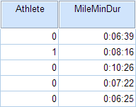
In the sample data, we will use two variables: Athlete and MileMinDur . The variable Athlete has values of either “0” (non-athlete) or "1" (athlete). It will function as the independent variable in this T test. The variable MileMinDur is a numeric duration variable (h:mm:ss), and it will function as the dependent variable. In SPSS, the first few rows of data look like this:

Before the Test

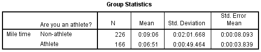
Before running the Independent Samples t Test, it is a good idea to look at descriptive statistics and graphs to get an idea of what to expect. Running Compare Means ( Analyze > Compare Means > Means ) to get descriptive statistics by group tells us that the standard deviation in mile time for non-athletes is about 2 minutes; for athletes, it is about 49 seconds. This corresponds to a variance of 14803 seconds for non-athletes, and a variance of 2447 seconds for athletes 1 . Running the Explore procedure ( Analyze > Descriptives > Explore ) to obtain a comparative boxplot yields the following graph:

If the variances were indeed equal, we would expect the total length of the boxplots to be about the same for both groups. However, from this boxplot, it is clear that the spread of observations for non-athletes is much greater than the spread of observations for athletes. Already, we can estimate that the variances for these two groups are quite different. It should not come as a surprise if we run the Independent Samples t Test and see that Levene's Test is significant.

Additionally, we should also decide on a significance level (typically denoted using the Greek letter alpha, α ) before we perform our hypothesis tests. The significance level is the threshold we use to decide whether a test result is significant. For this example, let's use α = 0.05.

1 When computing the variance of a duration variable (formatted as hh:mm:ss or mm:ss or mm:ss.s), SPSS converts the standard deviation value to seconds before squaring.

Running the Test

To run the Independent Samples t Test:

• Click  Analyze > Compare Means > Independent-Samples T Test .
• Move the variable Athlete to the Grouping Variable field, and move the variable MileMinDur to the Test Variable(s) area. Now Athlete is defined as the independent variable and MileMinDur is defined as the dependent variable.
• Click Define Groups , which opens a new window. Use specified values is selected by default. Since our grouping variable is numerically coded (0 = "Non-athlete", 1 = "Athlete"), type “0” in the first text box, and “1” in the second text box. This indicates that we will compare groups 0 and 1, which correspond to non-athletes and athletes, respectively. Click Continue when finished.
• Click OK to run the Independent Samples t Test. Output for the analysis will display in the Output Viewer window. 

Two sections (boxes) appear in the output: Group Statistics and Independent Samples Test . The first section, Group Statistics , provides basic information about the group comparisons, including the sample size ( n ), mean, standard deviation, and standard error for mile times by group. In this example, there are 166 athletes and 226 non-athletes. The mean mile time for athletes is 6 minutes 51 seconds, and the mean mile time for non-athletes is 9 minutes 6 seconds.

The second section, Independent Samples Test , displays the results most relevant to the Independent Samples t Test. There are two parts that provide different pieces of information: (A) Levene’s Test for Equality of Variances and (B) t-test for Equality of Means.

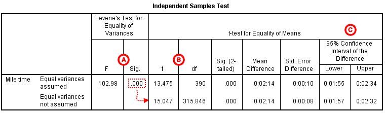
A Levene's Test for Equality of of Variances : This section has the test results for Levene's Test. From left to right:

• F is the test statistic of Levene's test
• Sig. is the p-value corresponding to this test statistic.

The p -value of Levene's test is printed as ".000" (but should be read as p < 0.001 -- i.e., p very small), so we we reject the null of Levene's test and conclude that the variance in mile time of athletes is significantly different than that of non-athletes. This tells us that we should look at the "Equal variances not assumed" row for the t test (and corresponding confidence interval) results . (If this test result had not been significant -- that is, if we had observed p > α -- then we would have used the "Equal variances assumed" output.)

B t-test for Equality of Means provides the results for the actual Independent Samples t Test. From left to right:

• t is the computed test statistic, using the formula for the equal-variances-assumed test statistic (first row of table) or the formula for the equal-variances-not-assumed test statistic (second row of table)
• df is the degrees of freedom, using the equal-variances-assumed degrees of freedom formula (first row of table) or the equal-variances-not-assumed degrees of freedom formula (second row of table)
• Sig (2-tailed) is the p-value corresponding to the given test statistic and degrees of freedom
• Mean Difference is the difference between the sample means, i.e. x 1  − x 2 ; it also corresponds to the numerator of the test statistic for that test
• Std. Error Difference is the standard error of the mean difference estimate; it also corresponds to the denominator of the test statistic for that test

Note that the mean difference is calculated by subtracting the mean of the second group from the mean of the first group. In this example, the mean mile time for athletes was subtracted from the mean mile time for non-athletes (9:06 minus 6:51 = 02:14). The sign of the mean difference corresponds to the sign of the t value. The positive t value in this example indicates that the mean mile time for the first group, non-athletes, is significantly greater than the mean for the second group, athletes.

The associated p value is printed as ".000"; double-clicking on the p-value will reveal the un-rounded number. SPSS rounds p-values to three decimal places, so any p-value too small to round up to .001 will print as .000. (In this particular example, the p-values are on the order of 10 -40 .)

C Confidence Interval of the Difference : This part of the t -test output complements the significance test results. Typically, if the CI for the mean difference contains 0 within the interval -- i.e., if the lower boundary of the CI is a negative number and the upper boundary of the CI is a positive number -- the results are not significant at the chosen significance level. In this example, the 95% CI is [01:57, 02:32], which does not contain zero; this agrees with the small p -value of the significance test.

Decision and Conclusions

Since p < .001 is less than our chosen significance level α = 0.05, we can reject the null hypothesis, and conclude that the that the mean mile time for athletes and non-athletes is significantly different.

Based on the results, we can state the following:

• There was a significant difference in mean mile time between non-athletes and athletes ( t 315.846 = 15.047, p < .001).
• The average mile time for athletes was 2 minutes and 14 seconds lower than the average mile time for non-athletes.
• << Previous: Paired Samples t Test
• Next: One-Way ANOVA >>
• Last Updated: Apr 10, 2024 4:50 PM
• URL: https://libguides.library.kent.edu/SPSS

Street Address

Mailing address, quick links.

• How Are We Doing?
• Student Jobs

Information

• Accessibility
• Emergency Information
• For Our Alumni
• For the Media
• Jobs & Employment
• Life at KSU
• Privacy Statement
• Technology Support
• Website Feedback

• school Campus Bookshelves
• menu_book Bookshelves
• perm_media Learning Objects
• login Login
• how_to_reg Request Instructor Account
• hub Instructor Commons
• Download Page (PDF)
• Download Full Book (PDF)
• Periodic Table
• Physics Constants
• Scientific Calculator
• Reference & Cite
• Tools expand_more
• Readability

selected template will load here

This action is not available.

8.2: Hypothesis Testing with t

• Last updated
• Save as PDF
• Page ID 7127

• Foster et al.
• University of Missouri-St. Louis, Rice University, & University of Houston, Downtown Campus via University of Missouri’s Affordable and Open Access Educational Resources Initiative

Hypothesis testing with the \(t\)-statistic works exactly the same way as \(z\)-tests did, following the four-step process of

• Stating the Hypothesis
• Finding the Critical Values
• Computing the Test Statistic
• Making the Decision.

We will work though an example: let’s say that you move to a new city and find a an auto shop to change your oil. Your old mechanic did the job in about 30 minutes (though you never paid close enough attention to know how much that varied), and you suspect that your new shop takes much longer. After 4 oil changes, you think you have enough evidence to demonstrate this.

Step 1: State the Hypotheses Our hypotheses for 1-sample t-tests are identical to those we used for \(z\)-tests. We still state the null and alternative hypotheses mathematically in terms of the population parameter and written out in readable English. For our example:

\(H_0\): There is no difference in the average time to change a car’s oil

\(H_0: μ = 30\)

\(H_A\): This shop takes longer to change oil than your old mechanic

\(H_A: μ > 30\)

Step 2: Find the Critical Values As noted above, our critical values still delineate the area in the tails under the curve corresponding to our chosen level of significance. Because we have no reason to change significance levels, we will use \(α\) = 0.05, and because we suspect a direction of effect, we have a one-tailed test. To find our critical values for \(t\), we need to add one more piece of information: the degrees of freedom. For this example:

\[df = N – 1 = 4 – 1 = 3 \nonumber \]

Going to our \(t\)-table, we find the column corresponding to our one-tailed significance level and find where it intersects with the row for 3 degrees of freedom. As shown in Figure \(\PageIndex{1}\): our critical value is \(t*\) = 2.353

We can then shade this region on our \(t\)-distribution to visualize our rejection region

Step 3: Compute the Test Statistic The four wait times you experienced for your oil changes are the new shop were 46 minutes, 58 minutes, 40 minutes, and 71 minutes. We will use these to calculate \(\overline{\mathrm{X}}\) and s by first filling in the sum of squares table in Table \(\PageIndex{1}\):

After filling in the first row to get \(\Sigma\)=215, we find that the mean is \(\overline{\mathrm{X}}\) = 53.75 (215 divided by sample size 4), which allows us to fill in the rest of the table to get our sum of squares \(SS\) = 564.74, which we then plug in to the formula for standard deviation from chapter 3:

\[s=\sqrt{\dfrac{\sum(X-\overline{X})^{2}}{N-1}}=\sqrt{\dfrac{S S}{d f}}=\sqrt{\dfrac{564.74}{3}}=13.72 \nonumber \]

Next, we take this value and plug it in to the formula for standard error:

\[s_{\overline{X}}=\dfrac{s}{\sqrt{n}}=\dfrac{13.72}{2}=6.86 \nonumber \]

And, finally, we put the standard error, sample mean, and null hypothesis value into the formula for our test statistic \(t\):

\[t=\dfrac{\overline{\mathrm{X}}-\mu}{s_{\overline{\mathrm{X}}}}=\dfrac{53.75-30}{6.86}=\dfrac{23.75}{6.68}=3.46 \nonumber \]

This may seem like a lot of steps, but it is really just taking our raw data to calculate one value at a time and carrying that value forward into the next equation: data  sample size/degrees of freedom  mean  sum of squares  standard deviation  standard error  test statistic. At each step, we simply match the symbols of what we just calculated to where they appear in the next formula to make sure we are plugging everything in correctly.

Step 4: Make the Decision Now that we have our critical value and test statistic, we can make our decision using the same criteria we used for a \(z\)-test. Our obtained \(t\)-statistic was \(t\) = 3.46 and our critical value was \(t* = 2.353: t > t*\), so we reject the null hypothesis and conclude:

Based on our four oil changes, the new mechanic takes longer on average (\(\overline{\mathrm{X}}\) = 53.75) to change oil than our old mechanic, \(t(3)\) = 3.46, \(p\) < .05.

Notice that we also include the degrees of freedom in parentheses next to \(t\). And because we found a significant result, we need to calculate an effect size, which is still Cohen’s \(d\), but now we use \(s\) in place of \(σ\):

\[d=\dfrac{\overline{X}-\mu}{s}=\dfrac{53.75-30.00}{13.72}=1.73 \nonumber \]

This is a large effect. It should also be noted that for some things, like the minutes in our current example, we can also interpret the magnitude of the difference we observed (23 minutes and 45 seconds) as an indicator of importance since time is a familiar metric.

7. The t tests

• The calculation of a confidence interval for a sample mean.
• The mean and standard deviation of a sample are calculated and a value is postulated for the mean of the population. How significantly does the sample mean differ from the postulated population mean?
• The means and standard deviations of two samples are calculated. Could both samples have been taken from the same population?
• Paired observations are made on two samples (or in succession on one sample). What is the significance of the difference between the means of the two sets of observations?

Confidence interval for the mean from a small sample

Statistical analysis and graphing software for scientists

Bioinformatics, cloning, and antibody discovery software

Plan, visualize, & document core molecular biology procedures

Electronic Lab Notebook to organize, search and share data

Proteomics software for analysis of mass spec data

Modern cytometry analysis platform

Analysis, statistics, graphing and reporting of flow cytometry data

Software to optimize designs of clinical trials

T test calculator

A t test compares the means of two groups. There are several types of two sample t tests and this calculator focuses on the three most common: unpaired, welch's, and paired t tests. Directions for using the calculator are listed below, along with more information about two sample t tests and help on which is appropriate for your analysis. NOTE: This is not the same as a one sample t test; for that, you need this One sample t test calculator .

1. Choose data entry format

Caution: Changing format will erase your data.

2. Choose a test

Help me choose

3. Enter data

Help me arrange the data

4. View the results

What is a t test.

A t test is used to measure the difference between exactly two means. Its focus is on the same numeric data variable rather than counts or correlations between multiple variables. If you are taking the average of a sample of measurements, t tests are the most commonly used method to evaluate that data. It is particularly useful for small samples of less than 30 observations. For example, you might compare whether systolic blood pressure differs between a control and treated group, between men and women, or any other two groups.

This calculator uses a two-sample t test, which compares two datasets to see if their means are statistically different. That is different from a one sample t test , which compares the mean of your sample to some proposed theoretical value.

The most general formula for a t test is composed of two means (M1 and M2) and the overall standard error (SE) of the two samples:

See our video on How to Perform a Two-sample t test for an intuitive explanation of t tests and an example.

How to use the t test calculator

• Choose your data entry format . This will change how section 3 on the page looks. The first two options are for entering your data points themselves, either manually or by copy & paste. The last two are for entering the means for each group, along with the number of observations (N) and either the standard error of that mean (SEM) or standard deviation of the dataset (SD) standard error. If you have already calculated these summary statistics, the latter options will save you time.
• Choose a test from the three options: Unpaired t test, Welch's unpaired t test, or Paired t test. Use our Ultimate Guide to t tests if you are unsure which is appropriate, as it includes a section on "How do I know which t test to use?". Notice not all options are available if you enter means only.
• Enter data for the test, based on the format you chose in Step 1.
• Click Calculate Now and View the results. All options will perform a two-tailed test .

Performing t tests? We can help.

Sign up for more information on how to perform t tests and other common statistical analyses.

Common t test confusion

In addition to the number of t test options, t tests are often confused with completely different techniques as well. Here's how to keep them all straight.

Correlation and regression are used to measure how much two factors move together. While t tests are part of regression analysis, they are focused on only one factor by comparing means in different samples.

ANOVA is used for comparing means across three or more total groups. In contrast, t tests compare means between exactly two groups.

Finally, contingency tables compare counts of observations within groups rather than a calculated average. Since t tests compare means of continuous variable between groups, contingency tables use methods such as chi square instead of t tests.

Assumptions of t tests

Because there are several versions of t tests, it's important to check the assumptions to figure out which is best suited for your project. Here are our analysis checklists for unpaired t tests and paired t tests , which are the two most common. These (and the ultimate guide to t tests ) go into detail on the basic assumptions underlying any t test:

• Exactly two groups
• Sample is normally distributed
• Independent observations
• Unequal or equal variance?
• Paired or unpaired data?

Interpreting results

The three different options for t tests have slightly different interpretations, but they all hinge on hypothesis testing and P values. You need to select a significance threshold for your P value (often 0.05) before doing the test.

While P values can be easy to misinterpret , they are the most commonly used method to evaluate whether there is evidence of a difference between the sample of data collected and the null hypothesis. Once you have run the correct t test, look at the resulting P value. If the test result is less than your threshold, you have enough evidence to conclude that the data are significantly different.

If the test result is larger or equal to your threshold, you cannot conclude that there is a difference. However, you cannot conclude that there was definitively no difference either. It's possible that a dataset with more observations would have resulted in a different conclusion.

Depending on the test you run, you may see other statistics that were used to calculate the P value, including the mean difference, t statistic, degrees of freedom, and standard error. The confidence interval and a review of your dataset is given as well on the results page.

Graphing t tests

This calculator does not provide a chart or graph of t tests, however, graphing is an important part of analysis because it can help explain the results of the t test and highlight any potential outliers. See our Prism guide for some graphing tips for both unpaired and paired t tests.

Prism is built for customized, publication quality graphics and charts. For t tests we recommend simply plotting the datapoints themselves and the mean, or an estimation plot . Another popular approach is to use a violin plot, like those available in Prism.

For more information

Our ultimate guide to t tests includes examples, links, and intuitive explanations on the subject. It is quite simply the best place to start if you're looking for more about t tests!

If you enjoyed this calculator, you will love using Prism for analysis. Take a free 30-day trial to do more with your data, such as:

• Clear guidance to pick the right t test and detailed results summaries
• Custom, publication quality t test graphics, violin plots, and more
• More t test options, including normality testing as well as nested and multiple t tests
• Non-parametric test alternatives such as Wilcoxon, Mann-Whitney, and Kolmogorov-Smirnov

Check out our video on how to perform a t test in Prism , for an example from start to finish!

Remember, this page is just for two sample t tests. If you only have one sample, you need to use this calculator instead.

We Recommend:

Analyze, graph and present your scientific work easily with GraphPad Prism. No coding required.