

Logistic regression
Logistic regression #.
We model the joint probability as:
This is the same as using a linear model for the log odds:
Fitting logistic regression #
The training data is a list of pairs \((y_1,x_1), (y_2,x_2), \dots, (y_n,x_n)\) .
We don’t observe the left hand side in the model
\(\implies\) We cannot use a least squares fit.
Likelihood #
Solution: The likelihood is the probability of the training data, for a fixed set of coefficients \(\beta_0,\dots,\beta_p\) :
We can rewrite as
Choose estimates \(\hat \beta_0, \dots,\hat \beta_p\) which maximize the likelihood.
Solved with numerical methods (e.g. Newton’s algorithm).
Logistic regression in R #
Inference for logistic regression #.
We can estimate the Standard Error of each coefficient.
The \(z\) -statistic is the equivalent of the \(t\) -statistic in linear regression:
The \(p\) -values are test of the null hypothesis \(\beta_j=0\) (Wald’s test).
Other possible hypothesis tests: likelihood ratio test (chi-square distribution).
Example: Predicting credit card default #
Predictors:
student : 1 if student, 0 otherwise
balance : credit card balance
income : person’s income.
Confounding #
In this dataset, there is confounding , but little collinearity.
Students tend to have higher balances. So, balance is explained by student , but not very well.
People with a high balance are more likely to default.
Among people with a given balance , students are less likely to default.
Results: predicting credit card default #
Fig. 16 Confounding in Default data #
Using only balance #
Using only student #, using both balance and student #, using all 3 predictors #, multinomial logistic regression #.
Extension of logistic regression to more than 2 categories
Suppose \(Y\) takes values in \(\{1,2,\dots,K\}\) , then we can use a linear model for the log odds against a baseline category (e.g. 1): for \(j \neq 1\)
In this case \(\beta \in \mathbb{R}^{p \times (K-1)}\) is a matrix of coefficients.
Some potential problems #
The coefficients become unstable when there is collinearity. Furthermore, this affects the convergence of the fitting algorithm.
When the classes are well separated, the coefficients become unstable. This is always the case when \(p\geq n-1\) . In this case, prediction error is low, but \(\hat{\beta}\) is very variable.

Logistic Regression and Survival Analysis
- 1
- | 2
- | 3
- | 4
- Contributing Authors:
- Learning Objectives
- Logistic Regression
- Why use logistic regression?
- Overview of Logistic Regression
Logistic Regression in R
- Survival Analysis
- Why use survival analysis?
- Overview of Survival Analysis
- Things we did not cover (or only touched on)
To perform logistic regression in R, you need to use the glm() function. Here, glm stands for "general linear model." Suppose we want to run the above logistic regression model in R, we use the following command:
> summary( glm( vomiting ~ age, family = binomial(link = logit) ) )
glm(formula = vomiting ~ age, family = binomial(link = logit))
Deviance Residuals:
Min 1Q Median 3Q Max
-1.0671 -1.0174 -0.9365 1.3395 1.9196
Coefficients:
Estimate Std. Error z value Pr(>|z|)
(Intercept) -0.141729 0.106206 -1.334 0.182
age -0.015437 0.003965 -3.893 9.89e-05 ***
Signif. codes: 0 '***' 0.001 '**' 0.01 '*' 0.05 '.' 0.1 ' ' 1
(Dispersion parameter for binomial family taken to be 1)
Null deviance: 1452.3 on 1093 degrees of freedom
Residual deviance: 1433.9 on 1092 degrees of freedom
AIC: 1437.9
Number of Fisher Scoring iterations: 4
To get the significance for the overall model we use the following command:
> 1-pchisq(1452.3-1433.9, 1093-1092)
[1] 1.79058e-05
The input to this test is:
- deviance of "null" model minus deviance of current model (can be thought of as "likelihood")
- degrees of freedom of the null model minus df of current model
This is analogous to the global F test for the overall significance of the model that comes automatically when we run the lm() command. This is testing the null hypothesis that the model is no better (in terms of likelihood) than a model fit with only the intercept term, i.e. that all beta terms are 0.
Thus the logistic model for these data is:
E[ odds(vomiting) ] = -0.14 – 0.02*age
This means that for a one-unit increase in age there is a 0.02 decrease in the log odds of vomiting. This can be translated to e -0.02 = 0.98. Groups of people in an age group one unit higher than a reference group have, on average, 0.98 times the odds of vomiting.
How do we test the association between vomiting and age?
- H 0 : There is no association between vomiting and age (the odds ratio is equal to 1).
- H a : There is an association between vomiting and age (the odds ratio is not equal to 1).
When testing the null hypothesis that there is no association between vomiting and age we reject the null hypothesis at the 0.05 alpha level ( z = -3.89, p-value = 9.89e-05).
On average, the odds of vomiting is 0.98 times that of identical subjects in an age group one unit smaller.
Finally, when we are looking at whether we should include a particular variable in our model (maybe it's a confounder), we can include it based on the "10% rule," where if the change in our estimate of interest changes more than 10% when we include the new covariate in the model, then we that new covariate in our model. When we do this in logistic regression, we compare the exponential of the betas, not the untransformed betas themselves!
|
Test the hypothesis that being nauseated was not associated with sex and age (hint: use a multiple logistic regression model). Test the overall hypothesis that there is no association between nausea and sex and age. Then test the individual main effects hypothesis (i.e. no association between sex and nausea after adjusting for age, and vice versa). |
return to top | previous page | next page

17.2 Inference for Logistic Regression
Statistical inference for logistic regression with one explanatory variable is similar to statistical inference for simple linear regression. We calculate estimates of the model parameters and standard errors for these estimates. Confidence intervals are formed in the usual way, but we use standard Normal -values rather than critical values from the distributions. The ratio of the estimate to the standard error is the basis for hypothesis tests.
Wald statistic
The statistic is sometimes called the Wald statistic. Output from some statistical software reports the significance test result in terms of the square of the statistic.
This statistic is called a chi-square statistic. When the null hypothesis is true, it has a distribution that is approximately a distribution with one degree of freedom, and the -value is calculated as . Because the square of a standard Normal random variable has a distribution with one degree of freedom, the statistic and the chi-square statistic give the same results for statistical inference.

chi-square statistic, p. 463
Confidence Intervals and Significance Tests for Logistic Regression
An approximate level confidence interval for the slope in the logistic regression model is
The ratio of the odds for a value of the explanatory variable equal to to the odds for a value of the explanatory variable equal to is the odds ratio . A level confidence interval for the odds ratio is obtained by transforming the confidence interval for the slope,
In these expressions is the standard Normal critical value with area between and .
To test the hypothesis , compute the test statistic
In terms of a random variable having the distribution with one degree of freedom, the -value for a test of against is approximately .
We have expressed the null hypothesis in terms of the slope because this form closely resembles what we studied in simple linear regression. In many applications, however, the results are expressed in terms of the odds ratio. A slope of 0 is the same as an odds ratio of 1, so we often express the null hypothesis of interest as “the odds ratio is 1.” This means that the two odds are equal and the explanatory variable is not useful for predicting the odds.
EXAMPLE 17.7 Computer Output for Tipping Study
CASE 17.1 Figure 17.3 gives the output from Minitab and SAS for the tipping study. The parameter estimates match those we calculated in Example 17.4 . The standard errors are 0.1107 and 0.2678. A 95% confidence interval for the slope is
We are 95% confident that the slope is between 0.3182 and 1.368. Both Minitab and SAS output provide the odds ratio estimate and 95% confidence interval. If this interval is not provided, it is easy to compute from the interval for the slope :

We conclude, “Servers wearing red are more likely to be tipped than servers wearing a different color ( , 95% to 3.928).”
It is standard to use 95% confidence intervals, and software often reports these intervals. A 95% confidence interval for the odds ratio also provides a test of the null hypothesis that the odds ratio is 1 at the 5% significance level. If the confidence interval does not include 1, we reject and conclude that the odds for the two groups are different; if the interval does include 1, the data do not provide enough evidence to distinguish the groups in this way.
Apply Your Knowledge
Question 17.8
17.8 Read the output.
CASE 17.1 Examine the Minitab and SAS output in Figure 17.3 . Create a table that reports the estimates of and with the standard errors. Also report the odds ratio with its 95% confidence interval as given in this output.
Question 17.9
17.9 Inference for energy drink commercials.
Use software to run a logistic regression analysis for the energy drink commercial data of Exercise 17.1 . Summarize the results of the inference.
. The odds ratio estimate is 1.227; the 95% confidence interval is (0.761, 1.979).
Question 17.10
17.10 Inference for audio/visual sharing.
Use software to run the logistic regression analysis for the audio/visual sharing data of Exercise 17.2 . Summarize the results of the inference.
Examples of logistic regression analyses
The following example is typical of many applications of logistic regression. It concerns a designed experiment with five different values for the explanatory variable.
EXAMPLE 17.8 Effectiveness of an Insecticide
As part of a cost-effectiveness study, a wholesale florist company ran an experiment to examine how well the insecticide rotenone kills an aphid called Macrosiphoniella sanborni that feeds on the chrysanthemum plant. 3 The explanatory variable is the concentration (in log of milligrams per liter) of the insecticide. About 50 aphids each were exposed to one of five concentrations. Each insect was either killed or not killed. Here are the data, along with the results of some calculations:
| Concentration (log scale) | Number of insects | Number killed | Proportion killed | Log odds |
| 0.96 | 50 | 6 | 0.1200 | −1.9924 |
| 1.33 | 48 | 16 | 0.3333 | −0.6931 |
| 1.63 | 46 | 24 | 0.5217 | 0.0870 |
| 2.04 | 49 | 42 | 0.8571 | 1.7918 |
| 2.32 | 50 | 44 | 0.8800 | 1.9924 |
Because there are replications at each concentration, we can calculate the proportion killed and estimate the log odds of death at each concentration. The logistic model in this case assumes that the log odds are linearly related to log concentration. Least-squares regression of log odds on log concentration gives the fit illustrated in Figure 17.4 . There is a clear linear relationship, which justifies our use of the logistic model. The logistic regression fit for the proportion killed appears in Figure 17.5 . It is a transformed version of Figure 17.4 with the fit calculated using the logistic model rather than least squares.

When the explanatory variable has several values, we can often use graphs like those in Figures 17.4 and 17.5 to visually assess whether the logistic regression model seems appropriate. Just as a scatterplot of y versus x in simple linear regression should show a linear pattern, a plot of log odds versus x in logistic regression should be close to linear. Just as in simple linear regression, outliers in the x direction should be avoided because they may overly influence the fitted model.
The graphs strongly suggest that insecticide concentration affects the kill rate in a way that fits the logistic regression model. Is the effect statistically significant ? Suppose that rotenone has no ability to kill Macrosiphoniella san-borni. What is the chance that we would observe experimental results at least as convincing as what we observed if this supposition were true? The answer is the -value for the test of the null hypothesis that the logistic regression slope is zero. If this -value is not small, our graph may be misleading. As usual, we must add inference to our data analysis.
EXAMPLE 17.9 Does Concentration Affect the Kill Rate?
Figure 17.6 gives the output from JMP and Minitab for logistic regression analysis of the insecticide data. The model is

where the values of the explanatory variable are 0.96, 1.33, 1.63, 2.04, 2.32. From the JMP output, we see that the fitted model is
Figure 17.5 is a graph of the fitted given by this equation against , along with the data used to fit the model. JMP gives the statistic under the heading “ChiSquare.” The null hypothesis that is clearly rejected ( , ).
The estimated odds ratio is 22.394. An increase of one unit in the log concentration of insecticide ( ) is associated with a 22-fold increase in the odds that an insect will be killed. The confidence interval for the odds is given in the Minitab output: (10.470, 47.896).
Remember that the test of the null hypothesis that the slope is 0 is the same as the test of the null hypothesis that the odds ratio is 1. If we were reporting the results in terms of the odds, we could say, “The odds of killing an insect increase by a factor of 22.3 for each unit increase in the log concentration of insecticide ( , ; 95% ).”
Question 17.11
17.11 Find the 95% confidence interval for the slope.
Using the information in the output of Figure 17.6 , find a 95% confidence interval for .
(2.349, 3.869).
Question 17.12
17.12 Find the 95% confidence interval for the odds ratio.
Using the estimate and its standard error in the output of Figure 17.6 , find the 95% confidence interval for the odds ratio and verify that this agrees with the interval given by Minitab.
Question 17.13
The Minitab output in Figure 17.6 does not give the value of . The column labeled “ -Value” provides similar information.
- Find the value under the heading “ -Value” for the predictor LCONC. Verify that this value is simply the estimated coefficient divided by its standard error. This is a statistic that has approximately the standard Normal distribution if the null hypothesis (slope 0) is true.
- Show that the square of is . The two-sided -value for is the same as for .
(a) . (b) 64.16, which agrees with the output up to rounding error.
In Example 17.6 , we studied the problem of predicting whether a movie will be profitable using the log opening-weekend revenue as the explanatory variable. We now revisit this example to include the results of inference.
EXAMPLE 17.10 Predicting a Movie's Profitability
Figure 17.7 gives the output from Minitab for a logistic regression analysis using log opening-weekend revenue as the explanatory variable. The fitted model is
This agrees up to rounding with the result reported in Example 17.6 .
From the output, we see that because , we cannot reject the null hypothesis that the slope . The value of the test statistic is , calculated from the estimate and its standard error . Minitab reports the odds ratio as 2.184, with a 95% confidence interval of (0.7584, 6.2898). Notice that this confidence interval contains the value 1, which is another way to assess . In this case, we don't have enough evidence to conclude that this explanatory variable, by itself, is helpful in predicting the probability that a movie will be profitable.

We estimate that a one-unit increase in the log opening-weekend revenue will increase the odds that the movie is profitable about 2.2 times. The data, however, do not give us a very accurate estimate. We do not have strong enough evidence to conclude that movies with higher opening-weekend revenues are more likely to be profitable. Establishing the true relationship accurately would require more data.
Companion to BER 642: Advanced Regression Methods
Chapter 11 multinomial logistic regression, 11.1 introduction to multinomial logistic regression.
Logistic regression is a technique used when the dependent variable is categorical (or nominal). For Binary logistic regression the number of dependent variables is two, whereas the number of dependent variables for multinomial logistic regression is more than two.
Examples: Consumers make a decision to buy or not to buy, a product may pass or fail quality control, there are good or poor credit risks, and employee may be promoted or not.
11.2 Equation
In logistic regression, a logistic transformation of the odds (referred to as logit) serves as the depending variable:
\[\log (o d d s)=\operatorname{logit}(P)=\ln \left(\frac{P}{1-P}\right)=a+b_{1} x_{1}+b_{2} x_{2}+b_{3} x_{3}+\ldots\]
\[p=\frac{\exp \left(a+b_{1} X_{1}+b_{2} X_{2}+b_{3} X_{3}+\ldots\right)}{1+\exp \left(a+b_{1} X_{1}+b_{2} X_{2}+b_{3} X_{3}+\ldots\right)}\] > Where:
p = the probability that a case is in a particular category,
exp = the exponential (approx. 2.72),
a = the constant of the equation and,
b = the coefficient of the predictor or independent variables.
Logits or Log Odds
Odds value can range from 0 to infinity and tell you how much more likely it is that an observation is a member of the target group rather than a member of the other group.
- Odds = p/(1-p)
If the probability is 0.80, the odds are 4 to 1 or .80/.20; if the probability is 0.25, the odds are .33 (.25/.75).
The odds ratio (OR), estimates the change in the odds of membership in the target group for a one unit increase in the predictor. It is calculated by using the regression coefficient of the predictor as the exponent or exp.
Assume in the example earlier where we were predicting accountancy success by a maths competency predictor that b = 2.69. Thus the odds ratio is exp(2.69) or 14.73. Therefore the odds of passing are 14.73 times greater for a student for example who had a pre-test score of 5 than for a student whose pre-test score was 4.
11.3 Hypothesis Test of Coefficients
In logistic regression, hypotheses are of interest:
The null hypothesis, which is when all the coefficients in the regression equation take the value zero, and
The alternate hypothesis that the model currently under consideration is accurate and differs significantly from the null of zero, i.e. gives significantly better than the chance or random prediction level of the null hypothesis.
Evaluation of Hypothesis
We then work out the likelihood of observing the data we actually did observe under each of these hypotheses. The result is usually a very small number, and to make it easier to handle, the natural logarithm is used, producing a log likelihood (LL) . Probabilities are always less than one, so LL’s are always negative. Log likelihood is the basis for tests of a logistic model.
11.4 Likelihood Ratio Test
The likelihood ratio test is based on -2LL ratio. It is a test of the significance of the difference between the likelihood ratio (-2LL) for the researcher’s model with predictors (called model chi square) minus the likelihood ratio for baseline model with only a constant in it.
Significance at the .05 level or lower means the researcher’s model with the predictors is significantly different from the one with the constant only (all ‘b’ coefficients being zero). It measures the improvement in fit that the explanatory variables make compared to the null model.
Chi square is used to assess significance of this ratio (see Model Fitting Information in SPSS output).
\(H_0\) : There is no difference between null model and final model.
\(H_1\) : There is difference between null model and final model.
11.5 Checking AssumptionL: Multicollinearity
Just run “linear regression” after assuming categorical dependent variable as continuous variable
If the largest VIF (Variance Inflation Factor) is greater than 10 then there is cause of concern (Bowerman & O’Connell, 1990)
Tolerance below 0.1 indicates a serious problem.
Tolerance below 0.2 indicates a potential problem (Menard,1995).
If the Condition index is greater than 15 then the multicollinearity is assumed.
11.6 Features of Multinomial logistic regression
Multinomial logistic regression to predict membership of more than two categories. It (basically) works in the same way as binary logistic regression. The analysis breaks the outcome variable down into a series of comparisons between two categories.
E.g., if you have three outcome categories (A, B and C), then the analysis will consist of two comparisons that you choose:
Compare everything against your first category (e.g. A vs. B and A vs. C),
Or your last category (e.g. A vs. C and B vs. C),
Or a custom category (e.g. B vs. A and B vs. C).
The important parts of the analysis and output are much the same as we have just seen for binary logistic regression.
11.7 R Labs: Running Multinomial Logistic Regression in R
11.7.1 understanding the data: choice of programs.
The data set(hsbdemo.sav) contains variables on 200 students. The outcome variable is prog, program type (1=general, 2=academic, and 3=vocational). The predictor variables are ses, social economic status (1=low, 2=middle, and 3=high), math, mathematics score, and science, science score: both are continuous variables.
(Research Question):When high school students choose the program (general, vocational, and academic programs), how do their math and science scores and their social economic status (SES) affect their decision?
11.7.2 Prepare and review the data
Now let’s do the descriptive analysis
11.7.3 Run the Multinomial Model using “nnet” package
Below we use the multinom function from the nnet package to estimate a multinomial logistic regression model. There are other functions in other R packages capable of multinomial regression. We chose the multinom function because it does not require the data to be reshaped (as the mlogit package does) and to mirror the example code found in Hilbe’s Logistic Regression Models.
First, we need to choose the level of our outcome that we wish to use as our baseline and specify this in the relevel function. Then, we run our model using multinom. The multinom package does not include p-value calculation for the regression coefficients, so we calculate p-values using Wald tests (here z-tests).
These are the logit coefficients relative to the reference category. For example,under ‘math’, the -0.185 suggests that for one unit increase in ‘science’ score, the logit coefficient for ‘low’ relative to ‘middle’ will go down by that amount, -0.185.
11.7.4 Check the model fit information
Interpretation of the Model Fit information
The log-likelihood is a measure of how much unexplained variability there is in the data. Therefore, the difference or change in log-likelihood indicates how much new variance has been explained by the model.
The chi-square test tests the decrease in unexplained variance from the baseline model (408.1933) to the final model (333.9036), which is a difference of 408.1933 - 333.9036 = 74.29. This change is significant, which means that our final model explains a significant amount of the original variability.
The likelihood ratio chi-square of 74.29 with a p-value < 0.001 tells us that our model as a whole fits significantly better than an empty or null model (i.e., a model with no predictors).
11.7.5 Calculate the Goodness of fit
11.7.6 calculate the pseudo r-square.
Interpretation of the R-Square:
These are three pseudo R squared values. Logistic regression does not have an equivalent to the R squared that is found in OLS regression; however, many people have tried to come up with one. These statistics do not mean exactly what R squared means in OLS regression (the proportion of variance of the response variable explained by the predictors), we suggest interpreting them with great caution.
Cox and Snell’s R-Square imitates multiple R-Square based on ‘likelihood’, but its maximum can be (and usually is) less than 1.0, making it difficult to interpret. Here it is indicating that there is the relationship of 31% between the dependent variable and the independent variables. Or it is indicating that 31% of the variation in the dependent variable is explained by the logistic model.
The Nagelkerke modification that does range from 0 to 1 is a more reliable measure of the relationship. Nagelkerke’s R2 will normally be higher than the Cox and Snell measure. In our case it is 0.357, indicating a relationship of 35.7% between the predictors and the prediction.
McFadden = {LL(null) – LL(full)} / LL(null). In our case it is 0.182, indicating a relationship of 18.2% between the predictors and the prediction.
11.7.7 Likelihood Ratio Tests
Interpretation of the Likelihood Ratio Tests
The results of the likelihood ratio tests can be used to ascertain the significance of predictors to the model. This table tells us that SES and math score had significant main effects on program selection, \(X^2\) (4) = 12.917, p = .012 for SES and \(X^2\) (2) = 10.613, p = .005 for SES.
These likelihood statistics can be seen as sorts of overall statistics that tell us which predictors significantly enable us to predict the outcome category, but they don’t really tell us specifically what the effect is. To see this we have to look at the individual parameter estimates.
11.7.8 Parameter Estimates
Note that the table is split into two rows. This is because these parameters compare pairs of outcome categories.
We specified the second category (2 = academic) as our reference category; therefore, the first row of the table labelled General is comparing this category against the ‘Academic’ category. the second row of the table labelled Vocational is also comparing this category against the ‘Academic’ category.
Because we are just comparing two categories the interpretation is the same as for binary logistic regression:
The relative log odds of being in general program versus in academic program will decrease by 1.125 if moving from the highest level of SES (SES = 3) to the lowest level of SES (SES = 1) , b = -1.125, Wald χ2(1) = -5.27, p <.001.
Exp(-1.1254491) = 0.3245067 means that when students move from the highest level of SES (SES = 3) to the lowest level of SES (1= SES) the odds ratio is 0.325 times as high and therefore students with the lowest level of SES tend to choose general program against academic program more than students with the highest level of SES.
The relative log odds of being in vocational program versus in academic program will decrease by 0.56 if moving from the highest level of SES (SES = 3) to the lowest level of SES (SES = 1) , b = -0.56, Wald χ2(1) = -2.82, p < 0.01.
Exp(-0.56) = 0.57 means that when students move from the highest level of SES (SES = 3) to the lowest level of SES (SES=1) the odds ratio is 0.57 times as high and therefore students with the lowest level of SES tend to choose vocational program against academic program more than students with the highest level of SES.
11.7.9 Interpretation of the Predictive Equation
Please check your slides for detailed information. You can find all the values on above R outcomes.
11.7.10 Build a classification table
11.8 supplementary learning materials.
Field, A (2013). Discovering statistics using IBM SPSS statistics (4th ed.). Los Angeles, CA: Sage Publications
Agresti, A. (1996). An introduction to categorical data analysis. New York, NY: Wiley & Sons.
IBM SPSS Regression 22.
Logistic Regression
Logistic regression is the extension of simple linear regression . Simple Linear regression is a statistical technique that is used to learn about the relationship between the dependent and independent variables. In Linear regression, dependent and independent variables are continuous in nature. For example, we could apply it to sale and marketing expenditure, where we want to predict sales based on marketing expenditure. Where the dependent variable(s) is dichotomous or binary in nature, we cannot use simple linear regression. Logistic regression is the statistical technique used to predict the relationship between predictors and predicted variables where the dependent variable is binary. Furthermore, where our dependent variable has two categories, we use binary logistic regression. If our dependent variable has more than two categories, it will be necessary to use multinomial logistic regression, whereas if our dependent variable is ordinal in nature, we use ordinal logistic regression.
In logistic regression, we assume one reference category with which we compare other variables for the probability of the occurrence of specific ‘events’ by fitting a logistic curve.
Like other regression techniques, logistic regression involves the use of two hypotheses:
1.A Null hypothesis : null hypothesis beta coefficient is equal to zero, and,
2. Alternative hypothesis : Alternative hypothesis assumes that beta coefficient is not equal to zero.
Logistic regression does not require that the relationship between the dependent variable and independent variable(s) be linear. Also, logistic regression does not require the error term to be normally distributed. Logistic regression assumes that the independent variables are interval scaled or binary in nature. However, logistic regression does not require the variance between the categorical variables. In logistic regression, normality is also not required. However, logistic regression does assume the absence of outliers.
There are some key differences in the methodologies and processes involved in simple vs. logistic regression. In the case of simple regression, ANOVA is used to evaluate the overall model fitness. Furthermore, R-square is used to evaluate the variance, as explained by the independent variable. Cox and Snell’s R 2 , Nagelkerke’s R 2 , McFadden’s R 2 , Pseudo-R 2 are alternatives to the R-square in logistic regression. Furthermore, we use the t-test to assess the significance of individual variables where simple regression is concerned. However, in the case of logistic regression, we use the Wald statistic to assess the significance of the independent variables. Instead of simple beta, exponential beta is used in logistic regression as the independent coefficient. Exponential beta provides an odd ratio for the dependent variable based on the independent variables. This essentially is a probability of an event occurring vs. not occurring.
Rule of thumb (Peduzzi et al, 1996) recommends that to estimate the logistic regression function, a minimum of 10 cases per independent variable is required to achieve reliable and meaningful results. For instance, where 10 independent variables are concerned, a minimum sample size of 100 with at least 10 cases per variable (once you take missing values and outliers into account) are permissible.
Click here for dissertation statistics help.

We work with graduate students every day and know what it takes to get your research approved.
- Address committee feedback
- Roadmap to completion
- Understand your needs and timeframe
Introduction to Statistics and Data Science
Chapter 18 logistic regression, 18.1 what is logistic regression used for.
Logistic regression is useful when we have a response variable which is categorical with only two categories. This might seem like it wouldn’t be especially useful, however with a little thought we can see that this is actually a very useful thing to know how to do. Here are some examples where we might use logistic regression .
- Predict whether a customer will visit your website again using browsing data
- Predict whether a voter will vote for the democratic candidate in an upcoming election using demographic and polling data
- Predict whether a patient given a surgery will survive for 5+ years after the surgery using health data
- Given the history of a stock, market trends predict if the closing price tomorrow will be higher or lower than today?
With many other possible examples. We can often phrase important questions as yes/no or (0-1) answers where we want to use some data to better predict the outcome. This is a simple case of what is called a classification problem in the machine learning/data science community. Given some information we want to use a computer to decide make a prediction which can be sorted into some finite number of outcomes.
18.2 GLM: Generalized Linear Models
Our linear regression techniques thus far have focused on cases where the response ( \(Y\) ) variable is continuous in nature. Recall, they take the form: \[ \begin{equation} Y_i=\alpha+ \sum_{j=1}^N \beta_j X_{ij} \end{equation} \] Where \(alpha\) is the intercept and \(\{\beta_1, \beta_2, ... \beta_N\}\) are the slope parameters for the explanatory variables ( \(\{X_1, X_2, ...X_N\}\) ). However, our outputs \(Y_i\) should give the probability that \(Y_i\) takes the value 1 given the \(X_j\) values. The right hand side of our model above will produce values in \(\mathbb{R}=(-\infty, \infty)\) while the left hand side should live in \([0,1]\) .
Therefore to use a model like this we need to transform our outputs from [0,1] to the whole real line \(\mathbb{R}\) .

\[y_i=g \left( \alpha+ \sum_{j=1}^N \beta_j X_{ij} \right)\]
18.3 A Starting Example
Let’s consider the shot logs data set again. We will use the shot distance column SHOT_DIST and the FGM columns for a logistic regression. The FGM column is 1 if the shot was made and 0 otherwise (perfect candidate for the response variable in a logistic regression). We expect that the further the shot is from the basket (SHOT_DIST) the less likely it will be that the shot is made (FGM=1).
To build this model in R we will use the glm() command and specify the link function we are using a the logit function.
\[logit(p)=0.392-0.04 \times SD \implies p=logit^{-1}(0.392-0.04 \times SD)\] So we can find the probability of a shot going in 12 feet from the basket as:
Here is a plot of the probability of a shot going in as a function of the distance from the basket using our best fit coefficients.

18.3.1 Confidence Intervals for the Parameters
A major point of this book is that you should never be satisfied with a single number summary in statistics. Rather than just considering a single best fit for our coefficients we should really form some confidence intervals for their values.
As we saw for simple regression we can look at the confidence intervals for our intercepts and slopes using the confint command.
Note, these values are still in the logit transformed scale.
18.4 Equivalence of Logistic Regression and Proportion Tests
Suppose we want to use the categorical variable of the individual player in our analysis. In the interest of keeping our tables and graphs visible we will limit our players to just those who took more than 820 shots in the data set.
| Name | Number of Shots |
|---|---|
| blake griffin | 878 |
| chris paul | 851 |
| damian lillard | 925 |
| gordon hayward | 833 |
| james harden | 1006 |
| klay thompson | 953 |
| kyle lowry | 832 |
| kyrie irving | 919 |
| lamarcus aldridge | 1010 |
| lebron james | 947 |
| mnta ellis | 1004 |
| nikola vucevic | 889 |
| rudy gay | 861 |
| russell westbrook | 943 |
| stephen curry | 941 |
| tyreke evans | 875 |
Now we can get a reduced data set with just these players.
Lets form a logistic regression using just a categorical variable as the explanatory variable. \[ \begin{equation} logit(p)=\beta Player \end{equation} \]
If we take the inverse logit of the coefficients we get the field goal percentage of the players in our data set.
Now suppose we want to see if the players in our data set truly differ in their field goal percentages or whether the differences we observe could just be caused by random effects. To do this we want to compare a model without the players information included with one that includes this information. Let’s create a null model to compare against our player model.
This null model contains no explanatory variables and takes the form: \[logit(p_i)=\alpha\]
Thus, the shooting percentage is not allowed to vary between the players. We find based on this data an overall field goal percentage of:
Now we may compare logistic regression models using the anova command in R.
The second line contains a p value of 2.33e-5 telling us to reject the null hypothesis that the two models are equivalent. So we found that knowledge of the player does matter in calculating the probability of a shot being made.
Notice we could have performed this analysis as a proportion test using the null that all players shooting percentages are the same \(p_1=p_2=...p_{15}\)
Notice the p-value obtained matches the logistic regression ANOVA almost exactly. Thus, a proportion test can be viewed as a special case of a logistic regression.
18.5 Example: Building a More Accurate Model
Now we can form a model for the shooting percentages using the individual players data:
\[ logit(p_i)=\alpha+\beta_1 SF+\beta_2DD+\beta_3 \text{player_dummy} \]
18.6 Example: Measuring Team Defense Using Logistic Regression
\[ logit(p_i)=\alpha+\beta_1 SD+\beta_2 \text{Team}+\beta_3 (\text{Team}) (SD) \] Since the team defending is a categorical variable R will store it as a dummy variable when forming the regression. Thus the first level of this variable will not appear in our regression (or more precisely it will be included in the intercept \(\alpha\) and slope \(\beta_1\) ). Before we run the model we can see which team will be missing.
The below plot shows the expected shooting percentages at each distance for the teams in the data set.

#Better Approach
Kahneman, Daniel. 2011. Thinking, Fast and Slow . Macmillan.
Wickham, Hadley, and Garrett Grolemund. 2016. R for Data Science: Import, Tidy, Transform, Visualize, and Model Data . " O’Reilly Media, Inc.".
Xie, Yihui. 2019. Bookdown: Authoring Books and Technical Documents with R Markdown . https://CRAN.R-project.org/package=bookdown .
A comprehensive comparison of goodness-of-fit tests for logistic regression models
- Original Paper
- Published: 30 August 2024
- Volume 34 , article number 175 , ( 2024 )
Cite this article

- Huiling Liu 1 ,
- Xinmin Li 2 ,
- Feifei Chen 3 ,
- Wolfgang Härdle 4 , 5 , 6 &
- Hua Liang 7
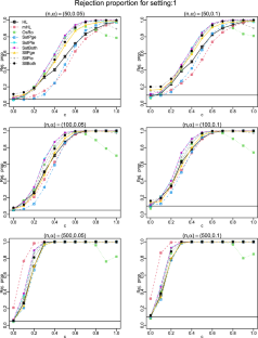
We introduce a projection-based test for assessing logistic regression models using the empirical residual marked empirical process and suggest a model-based bootstrap procedure to calculate critical values. We comprehensively compare this test and Stute and Zhu’s test with several commonly used goodness-of-fit (GoF) tests: the Hosmer–Lemeshow test, modified Hosmer–Lemeshow test, Osius–Rojek test, and Stukel test for logistic regression models in terms of type I error control and power performance in small ( \(n=50\) ), moderate ( \(n=100\) ), and large ( \(n=500\) ) sample sizes. We assess the power performance for two commonly encountered situations: nonlinear and interaction departures from the null hypothesis. All tests except the modified Hosmer–Lemeshow test and Osius–Rojek test have the correct size in all sample sizes. The power performance of the projection based test consistently outperforms its competitors. We apply these tests to analyze an AIDS dataset and a cancer dataset. For the former, all tests except the projection-based test do not reject a simple linear function in the logit, which has been illustrated to be deficient in the literature. For the latter dataset, the Hosmer–Lemeshow test, modified Hosmer–Lemeshow test, and Osius–Rojek test fail to detect the quadratic form in the logit, which was detected by the Stukel test, Stute and Zhu’s test, and the projection-based test.
This is a preview of subscription content, log in via an institution to check access.
Access this article
Subscribe and save.
- Get 10 units per month
- Download Article/Chapter or eBook
- 1 Unit = 1 Article or 1 Chapter
- Cancel anytime
Price includes VAT (Russian Federation)
Instant access to the full article PDF.
Rent this article via DeepDyve
Institutional subscriptions
A generalized Hosmer–Lemeshow goodness-of-fit test for a family of generalized linear models

Fifty Years with the Cox Proportional Hazards Regression Model

CPMCGLM: an R package for p -value adjustment when looking for an optimal transformation of a single explanatory variable in generalized linear models
Explore related subjects.
- Artificial Intelligence
Data availibility
No datasets were generated or analysed during the current study.
Chen, K., Hu, I., Ying, Z.: Strong consistency of maximum quasi-likelihood estimators in generalized linear models with fixed and adaptive designs. Ann. Stat. 27 (4), 1155–1163 (1999)
Article MathSciNet Google Scholar
Dardis, C.: LogisticDx: diagnostic tests and plots for logistic regression models. R package version 0.3 (2022)
Dikta, G., Kvesic, M., Schmidt, C.: Bootstrap approximations in model checks for binary data. J. Am. Stat. Assoc. 101 , 521–530 (2006)
Ekanem, I.A., Parkin, D.M.: Five year cancer incidence in Calabar, Nigeria (2009–2013). Cancer Epidemiol. 42 , 167–172 (2016)
Article Google Scholar
Escanciano, J.C.: A consistent diagnostic test for regression models using projections. Economet. Theor. 22 , 1030–1051 (2006)
Härdle, W., Mammen, E., Müller, M.: Testing parametric versus semiparametric modeling in generalized linear models. J. Am. Stat. Assoc. 93 , 1461–1474 (1998)
MathSciNet Google Scholar
Harrell, F.E.: rms: Regression modeling strategies. R package version 6.3-0 (2022)
Hosmer, D.W., Hjort, N.L.: Goodness-of-fit processes for logistic regression: simulation results. Stat. Med. 21 (18), 2723–2738 (2002)
Hosmer, D.W., Lemesbow, S.: Goodness of fit tests for the multiple logistic regression model. Commun Stat Theory Methods 9 , 1043–1069 (1980)
Hosmer, D.W., Hosmer, T., Le Cessie, S., Lemeshow, S.: A comparison of goodness-of-fit tests for the logistic regression model. Stat. Med. 16 (9), 965–980 (1997)
Hosmer, D., Lemeshow, S., Sturdivant, R.: Applied Logistic Regression. Wiley Series in Probability and Statistics, Wiley, New York (2013)
Book Google Scholar
Jones, L.K.: On a conjecture of Huber concerning the convergence of projection pursuit regression. Ann. Stat. 15 , 880–882 (1987)
Kohl, M.: MKmisc: miscellaneous functions from M. Kohl. R package version, vol. 1, p. 8 (2021)
Kosorok, M.R.: Introduction to Empirical Processes and Semiparametric Inference, vol. 61. Springer, New York (2008)
Lee, S.-M., Tran, P.-L., Li, C.-S.: Goodness-of-fit tests for a logistic regression model with missing covariates. Stat. Methods Med. Res. 31 , 1031–1050 (2022)
Lindsey, J.K.: Applying Generalized Linear Models. Springer, Berlin (2000)
McCullagh, P., Nelder, J.A.: Generalized Linear Models, vol. 37. Chapman and Hall (1989)
Nelder, J.A., Wedderburn, R.W.M.: Generalized linear models. J. R. Stat. Soc. Ser. A 135 , 370–384 (1972)
Oguntunde, P.E., Adejumo, A.O., Okagbue, H.I.: Breast cancer patients in Nigeria: data exploration approach. Data Brief 15 , 47 (2017)
Osius, G., Rojek, D.: Normal goodness-of-fit tests for multinomial models with large degrees of freedom. J. Am. Stat. Assoc. 87 (420), 1145–1152 (1992)
Rady, E.-H.A., Abonazel, M.R., Metawe’e, M.H.: A comparison study of goodness of fit tests of logistic regression in R: simulation and application to breast cancer data. Appl. Math. Sci. 7 , 50–59 (2021)
Google Scholar
Stukel, T.A.: Generalized logistic models. J. Am. Stat. Assoc. 83 (402), 426–431 (1988)
Stute, W., Zhu, L.-X.: Model checks for generalized linear models. Scand. J. Stat. Theory Appl. 29 , 535–545 (2002)
van der Vaart, A.W., Wellner, J.A.: Weak Convergence and Empirical Processes. Springer (1996)
van Heel, M., Dikta, G., Braekers, R.: Bootstrap based goodness-of-fit tests for binary multivariate regression models. J. Korean Stat. Soc. 51 (1), 308–335 (2022)
Yin, C., Zhao, L., Wei, C.: Asymptotic normality and strong consistency of maximum quasi-likelihood estimates in generalized linear models. Sci. China Ser. A Math. 49 , 145–157 (2006)
Download references
Acknowledgements
Li’s research was partially supported by NNSFC grant 11871294. Härdle gratefully acknowledges support through the European Cooperation in Science & Technology COST Action grant CA19130 - Fintech and Artificial Intelligence in Finance - Towards a transparent financial industry; the project “IDA Institute of Digital Assets”, CF166/15.11.2022, contract number CN760046/ 23.05.2024 financed under the Romanias National Recovery and Resilience Plan, Apel nr. PNRR-III-C9-2022-I8; and the Marie Skłodowska-Curie Actions under the European Union’s Horizon Europe research and innovation program for the Industrial Doctoral Network on Digital Finance, acronym DIGITAL, Project No. 101119635
Author information
Authors and affiliations.
Department of Statistics, South China University of Technology, Guangzhou, China
Huiling Liu
School of Mathematics and Statistics, Qingdao University, Shandong, 266071, China
Center for Statistics and Data Science, Beijing Normal University, Zhuhai, 519087, China
Feifei Chen
BRC Blockchain Research Center, Humboldt-Universität zu Berlin, 10178, Berlin, Germany
Wolfgang Härdle
Dept Information Management and Finance, National Yang Ming Chiao Tung U, Hsinchu, Taiwan
IDA Institute Digital Assets, Bucharest University of Economic Studies, Bucharest, Romania
Department of Statistics, George Washington University, Washington, DC, 20052, USA
You can also search for this author in PubMed Google Scholar
Contributions
LHL, LXM and LH wrote the main manuscript text, LHL and CFF program, HW commented on the methodological section. All authors reviewed the manuscript.
Corresponding author
Correspondence to Hua Liang .
Ethics declarations
Competing interests.
The authors declare no competing interests.
Additional information
Publisher's note.
Springer Nature remains neutral with regard to jurisdictional claims in published maps and institutional affiliations.
Rights and permissions
Springer Nature or its licensor (e.g. a society or other partner) holds exclusive rights to this article under a publishing agreement with the author(s) or other rightsholder(s); author self-archiving of the accepted manuscript version of this article is solely governed by the terms of such publishing agreement and applicable law.
Reprints and permissions
About this article
Liu, H., Li, X., Chen, F. et al. A comprehensive comparison of goodness-of-fit tests for logistic regression models. Stat Comput 34 , 175 (2024). https://doi.org/10.1007/s11222-024-10487-5
Download citation
Received : 02 December 2023
Accepted : 19 August 2024
Published : 30 August 2024
DOI : https://doi.org/10.1007/s11222-024-10487-5
Share this article
Anyone you share the following link with will be able to read this content:
Sorry, a shareable link is not currently available for this article.
Provided by the Springer Nature SharedIt content-sharing initiative
- Consistent test
- Model based bootstrap (MBB)
- Residual marked empirical process (RMEP)
- Find a journal
- Publish with us
- Track your research
Logistic regression
This page offers all the basic information you need about logistic regression analysis. It is part of Statkat’s wiki module, containing similarly structured info pages for many different statistical methods. The info pages give information about null and alternative hypotheses, assumptions, test statistics and confidence intervals, how to find p values, SPSS how-to’s and more.
To compare logistic regression analysis with other statistical methods, go to Statkat's Comparison tool or practice with logistic regression analysis at Statkat's Practice question center
- 1. When to use
- 2. Null hypothesis
- 3. Alternative hypothesis
- 4. Assumptions
- 5. Test statistic
- 6. Sampling distribution
- 7. Significant?
- 8. Wald-type approximate $C\%$ confidence interval for $\beta_k$
- 9. Goodness of fit measure $R^2_L$
- 10. Example context
When to use?
Note that theoretically, it is always possible to 'downgrade' the measurement level of a variable. For instance, a test that can be performed on a variable of ordinal measurement level can also be performed on a variable of interval measurement level, in which case the interval variable is downgraded to an ordinal variable. However, downgrading the measurement level of variables is generally a bad idea since it means you are throwing away important information in your data (an exception is the downgrade from ratio to interval level, which is generally irrelevant in data analysis).
If you are not sure which method you should use, you might like the assistance of our method selection tool or our method selection table .
Null hypothesis
Logistic regression analysis tests the following null hypothesis (H 0 ):
- H 0 : $\beta_1 = \beta_2 = \ldots = \beta_K = 0$
- H 0 : $\beta_k = 0$ or in terms of odds ratio:
- H 0 : $e^{\beta_k} = 1$
Alternative hypothesis
Logistic regression analysis tests the above null hypothesis against the following alternative hypothesis (H 1 or H a ):
- H 1 : not all population regression coefficients are 0
- H 1 : $\beta_k \neq 0$ or in terms of odds ratio:
- H 1 : $e^{\beta_k} \neq 1$ If defined as Wald $ = \dfrac{b_k}{SE_{b_k}}$ (see 'Test statistic'), also one sided alternatives can be tested:
- H 1 right sided: $\beta_k > 0$
- H 1 left sided: $\beta_k < 0$
- H 1 : $e^{\beta_k} \neq 1$
Assumptions
Statistical tests always make assumptions about the sampling procedure that was used to obtain the sample data. So called parametric tests also make assumptions about how data are distributed in the population. Non-parametric tests are more 'robust' and make no or less strict assumptions about population distributions, but are generally less powerful. Violation of assumptions may render the outcome of statistical tests useless, although violation of some assumptions (e.g. independence assumptions) are generally more problematic than violation of other assumptions (e.g. normality assumptions in combination with large samples).
Logistic regression analysis makes the following assumptions:
- In the population, the relationship between the independent variables and the log odds $\ln (\frac{\pi_{y=1}}{1 - \pi_{y=1}})$ is linear
- The residuals are independent of one another
- Variables are measured without error
- Multicollinearity
Test statistic
Logistic regression analysis is based on the following test statistic:
- $X^2 = D_{null} - D_K = \mbox{null deviance} - \mbox{model deviance} $ $D_{null}$, the null deviance, is conceptually similar to the total variance of the dependent variable in OLS regression analysis. $D_K$, the model deviance, is conceptually similar to the residual variance in OLS regression analysis.
- Wald $ = \dfrac{b_k^2}{SE^2_{b_k}}$
- Wald $ = \dfrac{b_k}{SE_{b_k}}$
- $X^2 = D_{K-1} - D_K$ $D_{K-1}$ is the model deviance, where independent variable $k$ is excluded from the model. $D_{K}$ is the model deviance, where independent variable $k$ is included in the model.
Sampling distribution
- chi-squared distribution with $K$ (number of independent variables) degrees of freedom
- If defined as Wald $ = \dfrac{b_k^2}{SE^2_{b_k}}$: approximately the chi-squared distribution with 1 degree of freedom
- If defined as Wald $ = \dfrac{b_k}{SE_{b_k}}$: approximately the standard normal distribution
- chi-squared distribution with 1 degree of freedom
Significant?
This is how you find out if your test result is significant:
- Check if $X^2$ observed in sample is equal to or larger than critical value $X^{2*}$ or
- Find $p$ value corresponding to observed $X^2$ and check if it is equal to or smaller than $\alpha$
- If defined as Wald $ = \dfrac{b_k^2}{SE^2_{b_k}}$: same procedure as for the chi-squared tests. Wald can be interpret as $X^2$
- If defined as Wald $ = \dfrac{b_k}{SE_{b_k}}$: same procedure as for any $z$ test. Wald can be interpreted as $z$.
Wald-type approximate $C\%$ confidence interval for $\beta_k$
Goodness of fit measure $r^2_l$, example context.
Logistic regression analysis could for instance be used to answer the question:
How to perform a logistic regression analysis in SPSS:
- Put your dependent variable in the box below Dependent and your independent (predictor) variables in the box below Covariate(s)
How to perform a logistic regression analysis in jamovi :
- Put your dependent variable in the box below Dependent Variable and your independent variables of interval/ratio level in the box below Covariates
- If you also have code (dummy) variables as independent variables, you can put these in the box below Covariates as well
- Instead of transforming your categorical independent variable(s) into code variables, you can also put the untransformed categorical independent variables in the box below Factors. Jamovi will then make the code variables for you 'behind the scenes'
- Skip to primary navigation
- Skip to main content
- Skip to primary sidebar
Statistical Methods and Data Analytics
Logistic Regression | SPSS Annotated Output
This page shows an example of logistic regression with footnotes explaining the output. These data were collected on 200 high schools students and are scores on various tests, including science, math, reading and social studies ( socst ). The variable female is a dichotomous variable coded 1 if the student was female and 0 if male.
In the syntax below, the get file command is used to load the hsb2 data into SPSS. In quotes, you need to specify where the data file is located on your computer. Remember that you need to use the .sav extension and that you need to end the command with a period. By default, SPSS does a listwise deletion of missing values. This means that only cases with non-missing values for the dependent as well as all independent variables will be used in the analysis.
Because we do not have a suitable dichotomous variable to use as our dependent variable, we will create one (which we will call honcomp , for honors composition) based on the continuous variable write . We do not advocate making dichotomous variables out of continuous variables; rather, we do this here only for purposes of this illustration.
Use the keyword with after the dependent variable to indicate all of the variables (both continuous and categorical) that you want included in the model. If you have a categorical variable with more than two levels, for example, a three-level ses variable (low, medium and high), you can use the categorical subcommand to tell SPSS to create the dummy variables necessary to include the variable in the logistic regression, as shown below. You can use the keyword by to create interaction terms. For example, the command logistic regression honcomp with read female read by female. will create a model with the main effects of read and female , as well as the interaction of read by female .
We will start by showing the SPSS commands to open the data file, creating the dichotomous dependent variable, and then running the logistic regression. We will show the entire output, and then break up the output with explanation.
Logistic Regression
Block 0: Beginning Block
Block 1: Method = Enter
This part of the output tells you about the cases that were included and excluded from the analysis, the coding of the dependent variable, and coding of any categorical variables listed on the categorical subcommand. (Note: You will not get the third table (“Categorical Variable Codings”) if you do not specify the categorical subcommand.)
b. N – This is the number of cases in each category (e.g., included in the analysis, missing, total).
c. Percent – This is the percent of cases in each category (e.g., included in the analysis, missing, total).
d. Included in Analysis – This row gives the number and percent of cases that were included in the analysis. Because we have no missing data in our example data set, this also corresponds to the total number of cases.
e. Missing Cases – This row give the number and percent of missing cases. By default, SPSS logistic regression does a listwise deletion of missing data. This means that if there is missing value for any variable in the model, the entire case will be excluded from the analysis.
f. Total – This is the sum of the cases that were included in the analysis and the missing cases. In our example, 200 + 0 = 200.
Unselected Cases – If the select subcommand is used and a logical condition is specified with a categorical variable in the dataset, then the number of unselected cases would be listed here. Using the select subcommand is different from using the filter command. When the select subcommand is used, diagnostic and residual values are computed for all cases in the data. If the filter command is used to select cases to be used in the analysis, residual and diagnostic values are not computed for unselected cases.
This part of the output describes a “null model”, which is model with no predictors and just the intercept. This is why you will see all of the variables that you put into the model in the table titled “Variables not in the Equation”.
c. Step 0 – SPSS allows you to have different steps in your logistic regression model. The difference between the steps is the predictors that are included. This is similar to blocking variables into groups and then entering them into the equation one group at a time. By default, SPSS logistic regression is run in two steps. The first step, called Step 0, includes no predictors and just the intercept. Often, this model is not interesting to researchers.
d. Observed – This indicates the number of 0’s and 1’s that are observed in the dependent variable.
e. Predicted – In this null model, SPSS has predicted that all cases are 0 on the dependent variable.
f. Overall Percentage – This gives the percent of cases for which the dependent variables was correctly predicted given the model. In this part of the output, this is the null model. 73.5 = 147/200.
g. B – This is the coefficient for the constant (also called the “intercept”) in the null model.
h. S.E. – This is the standard error around the coefficient for the constant.
i. Wald and Sig . – This is the Wald chi-square test that tests the null hypothesis that the constant equals 0. This hypothesis is rejected because the p-value (listed in the column called “Sig.”) is smaller than the critical p-value of .05 (or .01). Hence, we conclude that the constant is not 0. Usually, this finding is not of interest to researchers.
j. df – This is the degrees of freedom for the Wald chi-square test. There is only one degree of freedom because there is only one predictor in the model, namely the constant.
k. Exp(B) – This is the exponentiation of the B coefficient, which is an odds ratio. This value is given by default because odds ratios can be easier to interpret than the coefficient, which is in log-odds units. This is the odds: 53/147 = .361.
l. Score and Sig. – This is a Score test that is used to predict whether or not an independent variable would be significant in the model. Looking at the p-values (located in the column labeled “Sig.”), we can see that each of the predictors would be statistically significant except the first dummy for ses .
m. df – This column lists the degrees of freedom for each variable. Each variable to be entered into the model, e.g., read , science , ses(1) and ses(2) , has one degree of freedom, which leads to the total of four shown at the bottom of the column. The variable ses is listed here only to show that if the dummy variables that represent ses were tested simultaneously, the variable ses would be statistically significant.
n. Overall Statistics – This shows the result of including all of the predictors into the model.
The section contains what is frequently the most interesting part of the output: the overall test of the model (in the “Omnibus Tests of Model Coefficients” table) and the coefficients and odds ratios (in the “Variables in the Equation” table).
b. Step 1 – This is the first step (or model) with predictors in it. In this case, it is the full model that we specified in the logistic regression command. You can have more steps if you do stepwise or use blocking of variables.
c. Chi-square and Sig. – This is the chi-square statistic and its significance level. In this example, the statistics for the Step, Model and Block are the same because we have not used stepwise logistic regression or blocking. The value given in the Sig. column is the probability of obtaining the chi-square statistic given that the null hypothesis is true. In other words, this is the probability of obtaining this chi-square statistic (65.588) if there is in fact no effect of the independent variables, taken together, on the dependent variable. This is, of course, the p-value, which is compared to a critical value, perhaps .05 or .01 to determine if the overall model is statistically significant. In this case, the model is statistically significant because the p-value is less than .000.
d. df – This is the number of degrees of freedom for the model. There is one degree of freedom for each predictor in the model. In this example, we have four predictors: read , write and two dummies for ses (because there are three levels of ses ).
e. -2 Log likelihood – This is the -2 log likelihood for the final model. By itself, this number is not very informative. However, it can be used to compare nested (reduced) models.
f. Cox & Snell R Square and Nagelkerke R Square – These are pseudo R-squares. Logistic regression does not have an equivalent to the R-squared that is found in OLS regression; however, many people have tried to come up with one. There are a wide variety of pseudo-R-square statistics (these are only two of them). Because this statistic does not mean what R-squared means in OLS regression (the proportion of variance explained by the predictors), we suggest interpreting this statistic with great caution.
g. Observed – This indicates the number of 0’s and 1’s that are observed in the dependent variable.
h. Predicted – These are the predicted values of the dependent variable based on the full logistic regression model. This table shows how many cases are correctly predicted (132 cases are observed to be 0 and are correctly predicted to be 0; 27 cases are observed to be 1 and are correctly predicted to be 1), and how many cases are not correctly predicted (15 cases are observed to be 0 but are predicted to be 1; 26 cases are observed to be 1 but are predicted to be 0).
i. Overall Percentage – This gives the overall percent of cases that are correctly predicted by the model (in this case, the full model that we specified). As you can see, this percentage has increased from 73.5 for the null model to 79.5 for the full model.
j. B – These are the values for the logistic regression equation for predicting the dependent variable from the independent variable. They are in log-odds units. Similar to OLS regression, the prediction equation is
log(p/1-p) = b0 + b1*x1 + b2*x2 + b3*x3 + b3*x3+b4*x4
where p is the probability of being in honors composition. Expressed in terms of the variables used in this example, the logistic regression equation is
log(p/1-p) = –9.561 + 0.098*read + 0.066*science + 0.058*ses(1) – 1.013*ses(2)
These estimates tell you about the relationship between the independent variables and the dependent variable, where the dependent variable is on the logit scale. These estimates tell the amount of increase (or decrease, if the sign of the coefficient is negative) in the predicted log odds of honcomp = 1 that would be predicted by a 1 unit increase (or decrease) in the predictor, holding all other predictors constant. Note: For the independent variables which are not significant, the coefficients are not significantly different from 0, which should be taken into account when interpreting the coefficients. (See the columns labeled Wald and Sig. regarding testing whether the coefficients are statistically significant). Because these coefficients are in log-odds units, they are often difficult to interpret, so they are often converted into odds ratios. You can do this by hand by exponentiating the coefficient, or by looking at the right-most column in the Variables in the Equation table labeled “Exp(B)”. read – For every one-unit increase in reading score (so, for every additional point on the reading test), we expect a 0.098 increase in the log-odds of honcomp , holding all other independent variables constant. science – For every one-unit increase in science score, we expect a 0.066 increase in the log-odds of honcomp , holding all other independent variables constant. ses – This tells you if the overall variable ses is statistically significant. There is no coefficient listed, because ses is not a variable in the model. Rather, dummy variables which code for ses are in the equation, and those have coefficients. However, as you can see in this example, the coefficient for one of the dummies is statistically significant while the other one is not. The statistic given on this row tells you if the dummies that represent ses , taken together, are statistically significant. Because there are two dummies, this test has two degrees of freedom. This is equivalent to using the test statement in SAS or the test command is Stata. ses(1) – The reference group is level 3 (see the Categorical Variables Codings table above), so this coefficient represents the difference between level 1 of ses and level 3. Note: The number in the parentheses only indicate the number of the dummy variable; it does not tell you anything about which levels of the categorical variable are being compared. For example, if you changed the reference group from level 3 to level 1, the labeling of the dummy variables in the output would not change. ses(2) – The reference group is level 3 (see the Categorical Variables Codings table above), so this coefficient represents the difference between level 2 of ses and level 3. Note: The number in the parentheses only indicate the number of the dummy variable; it does not tell you anything about which levels of the categorical variable are being compared. For example, if you changed the reference group from level 3 to level 1, the labeling of the dummy variables in the output would not change. constant – This is the expected value of the log-odds of honcomp when all of the predictor variables equal zero. In most cases, this is not interesting. Also, oftentimes zero is not a realistic value for a variable to take.
k. S.E. – These are the standard errors associated with the coefficients. The standard error is used for testing whether the parameter is significantly different from 0; by dividing the parameter estimate by the standard error you obtain a t-value. The standard errors can also be used to form a confidence interval for the parameter.
l. Wald and Sig. – These columns provide the Wald chi-square value and 2-tailed p-value used in testing the null hypothesis that the coefficient (parameter) is 0. If you use a 2-tailed test, then you would compare each p-value to your preselected value of alpha. Coefficients having p-values less than alpha are statistically significant. For example, if you chose alpha to be 0.05, coefficients having a p-value of 0.05 or less would be statistically significant (i.e., you can reject the null hypothesis and say that the coefficient is significantly different from 0). If you use a 1-tailed test (i.e., you predict that the parameter will go in a particular direction), then you can divide the p-value by 2 before comparing it to your preselected alpha level. For the variable read , the p-value is .000, so the null hypothesis that the coefficient equals 0 would be rejected. For the variable science , the p-value is .015, so the null hypothesis that the coefficient equals 0 would be rejected. For the variable ses , the p-value is .035, so the null hypothesis that the coefficient equals 0 would be rejected. Because the test of the overall variable is statistically significant, you can look at the one degree of freedom tests for the dummies ses(1) and ses(2). The dummy ses(1) is not statistically significantly different from the dummy ses(3) (which is the omitted, or reference, category), but the dummy ses(2) is statistically significantly different from the dummy ses(3) with a p-value of .022.
m. df – This column lists the degrees of freedom for each of the tests of the coefficients.
n. Exp(B) – These are the odds ratios for the predictors. They are the exponentiation of the coefficients. There is no odds ratio for the variable ses because ses (as a variable with 2 degrees of freedom) was not entered into the logistic regression equation.
Odds Ratios
In this next example, we will illustrate the interpretation of odds ratios. In this example, we will simplify our model so that we have only one predictor, the binary variable female . Before we run the logistic regression, we will use the crosstabs command to obtain a crosstab of the two variables.
If we divide the number of males who are in honors composition, 18, by the number of males who are not in honors composition, 73, we get the odds of being in honors composition for males, 18/73 = .246. If we do the same thing for females, we get 35/74 = .472. To get the odds ratio, which is the ratio of the two odds that we have just calculated, we get .472/.246 = 1.918. As we can see in the output below, this is exactly the odds ratio we obtain from the logistic regression. The thing to remember here is that you want the group coded as 1 over the group coded as 0, so honcomp=1/honcomp=0 for both males and females, and then the odds for females/odds for males, because the females are coded as 1.
You can get the odds ratio from the crosstabs command by using the /statistics risk subcommand, as shown below.
As you can see in the output below, we get the same odds ratio when we run the logistic regression. (NOTE: Although it is equivalent to the odds ratio estimated from the logistic regression, the odds ratio in the “Risk Estimate” table is calculated as the ratio of the odds of honcomp=0 for males over the odds of honcomp=0 for females, which explains the confusing row heading “Odds Ratio for female (.00/1.00)”). If we calculated a 95% confidence interval, we would not want this to include the value of 1. When we were considering the coefficients, we did not want the confidence interval to include 0. If we exponentiate 0, we get 1 (exp(0) = 1). Hence, this is two ways of saying the same thing. As you can see, the 95% confidence interval includes 1; hence, the odds ratio is not statistically significant. Because the lower bound of the 95% confidence interval is so close to 1, the p-value is very close to .05. We can use the /print = ic(95) subcommand to get the 95% confidence intervals included in our output.
There are a few other things to note about the output below. The first is that although we have only one predictor variable, the test for the odds ratio does not match with the overall test of the model. This is because the test of the coefficient is a Wald chi-square test, while the test of the overall model is a likelihood ratio chi-square test. While these two types of chi-square tests are asymptotically equivalent, in small samples they can differ, as they do here. Also, we have the unfortunate situation in which the results of the two tests give different conclusions. This does not happen very often. In a situation like this, it is difficult to know what to conclude. One might consider the power, or one might decide if an odds ratio of this magnitude is important from a clinical or practical standpoint.
For more information on interpreting odds ratios, please see How do I interpret odds ratios in logistic regression? . Although this FAQ uses Stata for purposes of illustration, the concepts and explanations are useful.
Your Name (required)
Your Email (must be a valid email for us to receive the report!)
Comment/Error Report (required)
How to cite this page
- © 2024 UC REGENTS
Stack Exchange Network
Stack Exchange network consists of 183 Q&A communities including Stack Overflow , the largest, most trusted online community for developers to learn, share their knowledge, and build their careers.
Q&A for work
Connect and share knowledge within a single location that is structured and easy to search.
Wald test for logistic regression
As far as I understand the Wald test in the context of logistic regression is used to determine whether a certain predictor variable $X$ is significant or not. It rejects the null hypothesis of the corresponding coefficient being zero.
The test consists of dividing the value of the coefficient by standard error $\sigma$.
What I am confused about is that $X/\sigma$ is also known as Z-score and indicates how likely it is that a given observation comes form the normal distribution (with mean zero).
- z-statistic
- 2 $\begingroup$ Possible duplicate of Wald test in regression (OLS and GLMs): t- vs. z-distribution $\endgroup$ – Firebug Commented Nov 27, 2017 at 21:50
- 3 $\begingroup$ Perhaps it could be the other way around though, as the answer in this one is more developed. $\endgroup$ – Firebug Commented Nov 27, 2017 at 21:51
The estimates of the coefficients and the intercepts in logistic regression (and any GLM) are found via maximum-likelihood estimation (MLE). These estimates are denoted with a hat over the parameters, something like $\hat{\theta}$. Our parameter of interest is denoted $\theta_{0}$ and this is usually 0 as we want to test whether the coefficient differs from 0 or not. From asymptotic theory of MLE, we know that the difference between $\hat{\theta}$ and $\theta_{0}$ will be approximately normally distributed with mean 0 (details can be found in any mathematical statistics book such as Larry Wasserman's All of statistics ). Recall that standard errors are nothing else than standard deviations of statistics (Sokal and Rohlf write in their book Biometry : "a statistic is any one of many computed or estimated statistical quantities", e.g. the mean, median, standard deviation, correlation coefficient, regression coefficient, ...). Dividing a normal distribution with mean 0 and standard deviation $\sigma$ by its standard deviation will yield the standard normal distribution with mean 0 and standard deviation 1. The Wald statistic is defined as (e.g. Wasserman (2006): All of Statistics , pages 153, 214-215): $$ W=\frac{(\hat{\beta}-\beta_{0})}{\widehat{\operatorname{se}}(\hat{\beta})}\sim \mathcal{N}(0,1) $$ or $$ W^{2}=\frac{(\hat{\beta}-\beta_{0})^2}{\widehat{\operatorname{Var}}(\hat{\beta})}\sim \chi^{2}_{1} $$ The second form arises from the fact that the square of a standard normal distribution is the $\chi^{2}_{1}$-distribution with 1 degree of freedom (the sum of two squared standard normal distributions would be a $\chi^{2}_{2}$-distribution with 2 degrees of freedom and so on).
Because the parameter of interest is usually 0 (i.e. $\beta_{0}=0$), the Wald statistic simplifies to $$ W=\frac{\hat{\beta}}{\widehat{\operatorname{se}}(\hat{\beta})}\sim \mathcal{N}(0,1) $$ Which is what you described: The estimate of the coefficient divided by its standard error.
When is a $z$ and when a $t$ value used?
The choice between a $z$-value or a $t$-value depends on how the standard error of the coefficients has been calculated. Because the Wald statistic is asymptotically distributed as a standard normal distribution, we can use the $z$-score to calculate the $p$-value. When we, in addition to the coefficients, also have to estimate the residual variance, a $t$-value is used instead of the $z$-value. In ordinary least squares (OLS, normal linear regression), the variance-covariance matrix of the coefficients is $\operatorname{Var}[\hat{\beta}|X]=\sigma^2(X'X)^{-1}$ where $\sigma^2$ is the variance of the residuals (which is unknown and has to be estimated from the data) and $X$ is the design matrix . In OLS, the standard errors of the coefficients are the square roots of the diagonal elements of the variance-covariance matrix. Because we don't know $\sigma^2$, we have to replace it by its estimate $\hat{\sigma}^{2}=s^2$, so: $\widehat{\operatorname{se}}(\hat{\beta_{j}})=\sqrt{s^2(X'X)_{jj}^{-1}}$. Now that's the point: Because we have to estimate the variance of the residuals to calculate the standard error of the coefficients, we need to use a $t$-value and the $t$-distribution.
In logistic (and poisson) regression, the variance of the residuals is related to the mean. If $Y\sim Bin(n, p)$, the mean is $E(Y)=np$ and the variance is $\operatorname{Var}(Y)=np(1-p)$ so the variance and the mean are related. In logistic and poisson regression but not in regression with gaussian errors, we know the expected variance and don't have to estimate it separately. The dispersion parameter $\phi$ indicates if we have more or less than the expected variance. If $\phi=1$ this means we observe the expected amount of variance, whereas $\phi<1$ means that we have less than the expected variance (called underdispersion) and $\phi>1$ means that we have extra variance beyond the expected (called overdispersion). The dispersion parameter in logistic and poisson regression is fixed at 1 which means that we can use the $z$-score. The dispersion parameter . In other regression types such as normal linear regression, we have to estimate the residual variance and thus, a $t$-value is used for calculating the $p$-values. In R , look at these two examples:
Logistic regression
Note that the dispersion parameter is fixed at 1 and thus, we get $z$-values.
Normal linear regression (OLS)
Here, we have to estimate the residual variance (denoted as "Residual standard error") and hence, we use $t$-values instead of $z$-values. Of course, in large samples, the $t$-distribution approximates the normal distribution and the difference doesn't matter.
Another related post can be found here .
- 1 $\begingroup$ So, practically, regarding the first part of your excellent answer: If for some reason I'd have as an output the odds ratio and the Wald statistic, I could than calculate the standard error from these as: SE = (1/Wald-statistic)*ln(OR) Is this correct? Thanks! $\endgroup$ – Sander W. van der Laan Commented Aug 10, 2015 at 20:50
- 1 $\begingroup$ @SanderW.vanderLaan Thanks for your comment. Yes, I believe that's correct. If you perform a logistic regression, the Wald statistics will be the z-value. $\endgroup$ – COOLSerdash Commented Aug 11, 2015 at 16:13
- 2 $\begingroup$ Such a great answer!!. I do have some revision suggestions: I personally feel this answer is mixing up details with the punch lists. I would put the details of how linear regression is using variance of residuals in a separate graph. $\endgroup$ – Haitao Du Commented Apr 9, 2017 at 1:56
- 1 $\begingroup$ Also for dispersion parameter and the connection to the R code, may be we can open another section or a separation line to talk about. $\endgroup$ – Haitao Du Commented Apr 9, 2017 at 1:58
- 1 $\begingroup$ Just a side note about this answer: the specific formula given for the variance-covariance matrix is from ordinary least squares regression, not from logistic regression, which does not use the residual standard error but instead involves a diagonal matrix with the individual Bernoulli variances from the predicted probability for each observation along the diagonal. $\endgroup$ – ely Commented Aug 9, 2018 at 18:39
Not the answer you're looking for? Browse other questions tagged logistic z-statistic or ask your own question .
- Featured on Meta
- Announcing a change to the data-dump process
- Bringing clarity to status tag usage on meta sites
Hot Network Questions
- Testing if a string is a hexadecimal string in LaTeX3: code review, optimization, expandability, and protection
- Why is notation in logic so different from algebra?
- Possible thermal insulator to allow Unicellular organisms to survive a Venus like environment?
- Why are IBM's basis gates not linearly independent?
- Why is there so much salt in cheese?
- What is the difference between negation-eliminiation ¬E and contradiction-introduction ⊥I?
- Directory of Vegan Communities in Ecuador (South America)
- Getting an UK Visa with Ricevuta
- Using rule-based symbology for overlapping layers in QGIS
- Is the set of all non-computable numbers closed under addition?
- Can I arxive a paper that I had already published in a journal(EPL, in my case), so that eveyone can access it?
- Is there more evidence for god than for Russell’s teapot?
- What other marketable uses are there for Starship if Mars colonization falls through?
- How to run only selected lines of a shell script?
- Does a representation of the universal cover of a Lie group induce a projective representation of the group itself?
- Applying for different jobs finding out it is for the same project between different companies
- How would you slow the speed of a rogue solar system?
- Nearly stalled on takeoff after just 3 hours training on a PPL. Is this normal?
- Alternative to a single high spec'd diode
- Whats the safest way to store a password in database?
- Combination lock on a triangular rotating table
- What is the difference between passing NULL vs. nullptr to a template parameter?
- Do all instances of a given string get replaced under a rewrite rule?
- In Lord Rosse's 1845 drawing of M51, was the galaxy depicted in white or black?
Thank you for visiting nature.com. You are using a browser version with limited support for CSS. To obtain the best experience, we recommend you use a more up to date browser (or turn off compatibility mode in Internet Explorer). In the meantime, to ensure continued support, we are displaying the site without styles and JavaScript.
- View all journals
- Explore content
- About the journal
- Publish with us
- Sign up for alerts
- Published: 04 September 2024
CDK5–cyclin B1 regulates mitotic fidelity
- Xiao-Feng Zheng ORCID: orcid.org/0000-0001-8769-4604 1 na1 ,
- Aniruddha Sarkar ORCID: orcid.org/0000-0002-9393-1335 1 na1 ,
- Humphrey Lotana 2 ,
- Aleem Syed ORCID: orcid.org/0000-0001-7942-3900 1 ,
- Huy Nguyen ORCID: orcid.org/0000-0002-4424-1047 1 ,
- Richard G. Ivey 3 ,
- Jacob J. Kennedy 3 ,
- Jeffrey R. Whiteaker 3 ,
- Bartłomiej Tomasik ORCID: orcid.org/0000-0001-5648-345X 1 , 4 nAff7 ,
- Kaimeng Huang ORCID: orcid.org/0000-0002-0552-209X 1 , 5 ,
- Feng Li 1 ,
- Alan D. D’Andrea ORCID: orcid.org/0000-0001-6168-6294 1 , 5 ,
- Amanda G. Paulovich ORCID: orcid.org/0000-0001-6532-6499 3 ,
- Kavita Shah 2 ,
- Alexander Spektor ORCID: orcid.org/0000-0002-1085-3205 1 , 5 &
- Dipanjan Chowdhury ORCID: orcid.org/0000-0001-5645-3752 1 , 5 , 6
Nature ( 2024 ) Cite this article
Metrics details
CDK1 has been known to be the sole cyclin-dependent kinase (CDK) partner of cyclin B1 to drive mitotic progression 1 . Here we demonstrate that CDK5 is active during mitosis and is necessary for maintaining mitotic fidelity. CDK5 is an atypical CDK owing to its high expression in post-mitotic neurons and activation by non-cyclin proteins p35 and p39 2 . Here, using independent chemical genetic approaches, we specifically abrogated CDK5 activity during mitosis, and observed mitotic defects, nuclear atypia and substantial alterations in the mitotic phosphoproteome. Notably, cyclin B1 is a mitotic co-factor of CDK5. Computational modelling, comparison with experimentally derived structures of CDK–cyclin complexes and validation with mutational analysis indicate that CDK5–cyclin B1 can form a functional complex. Disruption of the CDK5–cyclin B1 complex phenocopies CDK5 abrogation in mitosis. Together, our results demonstrate that cyclin B1 partners with both CDK5 and CDK1, and CDK5–cyclin B1 functions as a canonical CDK–cyclin complex to ensure mitotic fidelity.
This is a preview of subscription content, access via your institution
Access options
Access Nature and 54 other Nature Portfolio journals
Get Nature+, our best-value online-access subscription
24,99 € / 30 days
cancel any time
Subscribe to this journal
Receive 51 print issues and online access
185,98 € per year
only 3,65 € per issue
Buy this article
- Purchase on SpringerLink
- Instant access to full article PDF
Prices may be subject to local taxes which are calculated during checkout

Core control principles of the eukaryotic cell cycle

CDC7-independent G1/S transition revealed by targeted protein degradation

Evolution of opposing regulatory interactions underlies the emergence of eukaryotic cell cycle checkpoints
Data availability.
All data supporting the findings of this study are available in the Article and its Supplementary Information . The LC–MS/MS proteomics data have been deposited to the ProteomeXchange Consortium 60 via the PRIDE 61 partner repository under dataset identifier PXD038386 . Correspondence regarding experiments and requests for materials should be addressed to the corresponding authors.
Wieser, S. & Pines, J. The biochemistry of mitosis. Cold Spring Harb. Perspect. Biol. 7 , a015776 (2015).
Article PubMed PubMed Central Google Scholar
Dhavan, R. & Tsai, L. H. A decade of CDK5. Nat. Rev. Mol. Cell Biol. 2 , 749–759 (2001).
Article CAS PubMed Google Scholar
Malumbres, M. Cyclin-dependent kinases. Genome Biol. 15 , 122 (2014).
Coverley, D., Laman, H. & Laskey, R. A. Distinct roles for cyclins E and A during DNA replication complex assembly and activation. Nat. Cell Biol. 4 , 523–528 (2002).
Desai, D., Wessling, H. C., Fisher, R. P. & Morgan, D. O. Effects of phosphorylation by CAK on cyclin binding by CDC2 and CDK2. Mol. Cell. Biol. 15 , 345–350 (1995).
Article CAS PubMed PubMed Central Google Scholar
Brown, N. R. et al. CDK1 structures reveal conserved and unique features of the essential cell cycle CDK. Nat. Commun. 6 , 6769 (2015).
Article ADS CAS PubMed PubMed Central Google Scholar
Strauss, B. et al. Cyclin B1 is essential for mitosis in mouse embryos, and its nuclear export sets the time for mitosis. J. Cell Biol. 217 , 179–193 (2018).
Gavet, O. & Pines, J. Activation of cyclin B1-Cdk1 synchronizes events in the nucleus and the cytoplasm at mitosis. J. Cell Biol. 189 , 247–259 (2010).
Barbiero, M. et al. Cell cycle-dependent binding between cyclin B1 and Cdk1 revealed by time-resolved fluorescence correlation spectroscopy. Open Biol. 12 , 220057 (2022).
Pines, J. & Hunter, T. Isolation of a human cyclin cDNA: evidence for cyclin mRNA and protein regulation in the cell cycle and for interaction with p34cdc2. Cell 58 , 833–846 (1989).
Clute, P. & Pines, J. Temporal and spatial control of cyclin B1 destruction in metaphase. Nat. Cell Biol. 1 , 82–87 (1999).
Potapova, T. A. et al. The reversibility of mitotic exit in vertebrate cells. Nature 440 , 954–958 (2006).
Basu, S., Greenwood, J., Jones, A. W. & Nurse, P. Core control principles of the eukaryotic cell cycle. Nature 607 , 381–386 (2022).
Santamaria, D. et al. Cdk1 is sufficient to drive the mammalian cell cycle. Nature 448 , 811–815 (2007).
Article ADS CAS PubMed Google Scholar
Zheng, X. F. et al. A mitotic CDK5-PP4 phospho-signaling cascade primes 53BP1 for DNA repair in G1. Nat. Commun. 10 , 4252 (2019).
Article ADS PubMed PubMed Central Google Scholar
Fagerberg, L. et al. Analysis of the human tissue-specific expression by genome-wide integration of transcriptomics and antibody-based proteomics. Mol. Cell. Proteom. 13 , 397–406 (2014).
Article CAS Google Scholar
Pozo, K. & Bibb, J. A. The emerging role of Cdk5 in cancer. Trends Cancer 2 , 606–618 (2016).
Sharma, S. & Sicinski, P. A kinase of many talents: non-neuronal functions of CDK5 in development and disease. Open Biol. 10 , 190287 (2020).
Sun, K. H. et al. Novel genetic tools reveal Cdk5’s major role in Golgi fragmentation in Alzheimer’s disease. Mol. Biol. Cell 19 , 3052–3069 (2008).
Sharma, S. et al. Targeting the cyclin-dependent kinase 5 in metastatic melanoma. Proc. Natl Acad. Sci. USA 117 , 8001–8012 (2020).
Nabet, B. et al. The dTAG system for immediate and target-specific protein degradation. Nat. Chem. Biol. 14 , 431–441 (2018).
Simpson, L. M. et al. Target protein localization and its impact on PROTAC-mediated degradation. Cell Chem. Biol. 29 , 1482–1504 e1487 (2022).
Vassilev, L. T. et al. Selective small-molecule inhibitor reveals critical mitotic functions of human CDK1. Proc. Natl Acad. Sci. USA 103 , 10660–10665 (2006).
Janssen, A. F. J., Breusegem, S. Y. & Larrieu, D. Current methods and pipelines for image-based quantitation of nuclear shape and nuclear envelope abnormalities. Cells 11 , 347 (2022).
Thompson, S. L. & Compton, D. A. Chromosome missegregation in human cells arises through specific types of kinetochore-microtubule attachment errors. Proc. Natl Acad. Sci. USA 108 , 17974–17978 (2011).
Kline-Smith, S. L. & Walczak, C. E. Mitotic spindle assembly and chromosome segregation: refocusing on microtubule dynamics. Mol. Cell 15 , 317–327 (2004).
Prosser, S. L. & Pelletier, L. Mitotic spindle assembly in animal cells: a fine balancing act. Nat. Rev. Mol. Cell Biol. 18 , 187–201 (2017).
Zeng, X. et al. Pharmacologic inhibition of the anaphase-promoting complex induces a spindle checkpoint-dependent mitotic arrest in the absence of spindle damage. Cancer Cell 18 , 382–395 (2010).
Warren, J. D., Orr, B. & Compton, D. A. A comparative analysis of methods to measure kinetochore-microtubule attachment stability. Methods Cell. Biol. 158 , 91–116 (2020).
Gregan, J., Polakova, S., Zhang, L., Tolic-Norrelykke, I. M. & Cimini, D. Merotelic kinetochore attachment: causes and effects. Trends Cell Biol 21 , 374–381 (2011).
Etemad, B., Kuijt, T. E. & Kops, G. J. Kinetochore-microtubule attachment is sufficient to satisfy the human spindle assembly checkpoint. Nat. Commun. 6 , 8987 (2015).
Tauchman, E. C., Boehm, F. J. & DeLuca, J. G. Stable kinetochore-microtubule attachment is sufficient to silence the spindle assembly checkpoint in human cells. Nat. Commun. 6 , 10036 (2015).
Mitchison, T. & Kirschner, M. Microtubule assembly nucleated by isolated centrosomes. Nature 312 , 232–237 (1984).
Fourest-Lieuvin, A. et al. Microtubule regulation in mitosis: tubulin phosphorylation by the cyclin-dependent kinase Cdk1. Mol. Biol. Cell 17 , 1041–1050 (2006).
Ubersax, J. A. et al. Targets of the cyclin-dependent kinase Cdk1. Nature 425 , 859–864 (2003).
Yang, C. H., Lambie, E. J. & Snyder, M. NuMA: an unusually long coiled-coil related protein in the mammalian nucleus. J. Cell Biol. 116 , 1303–1317 (1992).
Yang, C. H. & Snyder, M. The nuclear-mitotic apparatus protein is important in the establishment and maintenance of the bipolar mitotic spindle apparatus. Mol. Biol. Cell 3 , 1259–1267 (1992).
Kotak, S., Busso, C. & Gonczy, P. NuMA phosphorylation by CDK1 couples mitotic progression with cortical dynein function. EMBO J. 32 , 2517–2529 (2013).
Kitagawa, M. et al. Cdk1 coordinates timely activation of MKlp2 kinesin with relocation of the chromosome passenger complex for cytokinesis. Cell Rep. 7 , 166–179 (2014).
Schrock, M. S. et al. MKLP2 functions in early mitosis to ensure proper chromosome congression. J. Cell Sci. 135 , jcs259560 (2022).
Sun, M. et al. NuMA regulates mitotic spindle assembly, structural dynamics and function via phase separation. Nat. Commun. 12 , 7157 (2021).
Chen, Q., Zhang, X., Jiang, Q., Clarke, P. R. & Zhang, C. Cyclin B1 is localized to unattached kinetochores and contributes to efficient microtubule attachment and proper chromosome alignment during mitosis. Cell Res. 18 , 268–280 (2008).
Kabeche, L. & Compton, D. A. Cyclin A regulates kinetochore microtubules to promote faithful chromosome segregation. Nature 502 , 110–113 (2013).
Hegarat, N. et al. Cyclin A triggers mitosis either via the Greatwall kinase pathway or cyclin B. EMBO J. 39 , e104419 (2020).
Jumper, J. et al. Highly accurate protein structure prediction with AlphaFold. Nature 596 , 583–589 (2021).
Wood, D. J. & Endicott, J. A. Structural insights into the functional diversity of the CDK-cyclin family. Open Biol. 8 , 180112 (2018).
Brown, N. R., Noble, M. E., Endicott, J. A. & Johnson, L. N. The structural basis for specificity of substrate and recruitment peptides for cyclin-dependent kinases. Nat. Cell Biol. 1 , 438–443 (1999).
Tarricone, C. et al. Structure and regulation of the CDK5-p25 nck5a complex. Mol. Cell 8 , 657–669 (2001).
Poon, R. Y., Lew, J. & Hunter, T. Identification of functional domains in the neuronal Cdk5 activator protein. J. Biol. Chem. 272 , 5703–5708 (1997).
Oppermann, F. S. et al. Large-scale proteomics analysis of the human kinome. Mol. Cell. Proteom. 8 , 1751–1764 (2009).
van den Heuvel, S. & Harlow, E. Distinct roles for cyclin-dependent kinases in cell cycle control. Science 262 , 2050–2054 (1993).
Article ADS PubMed Google Scholar
Nakatani, Y. & Ogryzko, V. Immunoaffinity purification of mammalian protein complexes. Methods Enzymol. 370 , 430–444 (2003).
Tyanova, S., Temu, T. & Cox, J. The MaxQuant computational platform for mass spectrometry-based shotgun proteomics. Nat. Protoc. 11 , 2301–2319 (2016).
Tyanova, S. et al. The Perseus computational platform for comprehensive analysis of (prote)omics data. Nat. Methods 13 , 731–740 (2016).
Ritchie, M. E. et al. limma powers differential expression analyses for RNA-sequencing and microarray studies. Nucleic Acids Res. 43 , e47 (2015).
R Core Team. R: a language and environment for statistical computing (2021).
Wickham, H. ggplot2: elegant graphics for data analysis (2016).
Slowikowski, K. ggrepel: automatically position non-overlapping text labels with “ggplot2” (2018).
Wu, T. et al. clusterProfiler 4.0: a universal enrichment tool for interpreting omics data. Innovation 2 , 100141 (2021).
CAS PubMed PubMed Central Google Scholar
Deutsch, E. W. et al. The ProteomeXchange consortium in 2020: enabling ‘big data’ approaches in proteomics. Nucleic Acids Res. 48 , D1145–D1152 (2020).
CAS PubMed Google Scholar
Perez-Riverol, Y. et al. The PRIDE database and related tools and resources in 2019: improving support for quantification data. Nucleic Acids Res. 47 , D442–D450 (2019).
Robinson, M. D., McCarthy, D. J. & Smyth, G. K. edgeR: a Bioconductor package for differential expression analysis of digital gene expression data. Bioinformatics 26 , 139–140 (2010).
Nagahara, H. et al. Transduction of full-length TAT fusion proteins into mammalian cells: TAT-p27Kip1 induces cell migration. Nat. Med. 4 , 1449–1452 (1998).
Mirdita, M. et al. ColabFold: making protein folding accessible to all. Nat. Methods 19 , 679–682 (2022).
Lu, C. et al. OPLS4: improving force field accuracy on challenging regimes of chemical space. J. Chem. Theory Comput. 17 , 4291–4300 (2021).
Obenauer, J. C., Cantley, L. C. & Yaffe, M. B. Scansite 2.0: proteome-wide prediction of cell signaling interactions using short sequence motifs. Nucleic Acids Res. 31 , 3635–3641 (2003).
Download references
Acknowledgements
We thank D. Pellman for comments on the manuscript; W. Michowski, S. Sharma, P. Sicinski, B. Nabet and N. Gray for the reagents; J. A. Tainer for providing access to software used for structural analysis; and S. Gerber for sharing unpublished results. D.C. is supported by grants R01 CA208244 and R01 CA264900, DOD Ovarian Cancer Award W81XWH-15-0564/OC140632, Tina’s Wish Foundation, Detect Me If You Can, a V Foundation Award, a Gray Foundation grant and the Claudia Adams Barr Program in Innovative Basic Cancer Research. A. Spektor would like to acknowledge support from K08 CA208008, the Burroughs Wellcome Fund Career Award for Medical Scientists, Saverin Breast Cancer Research Fund and the Claudia Adams Barr Program in Innovative Basic Cancer Research. X.-F.Z. was an American Cancer Society Fellow and is supported by the Breast and Gynecologic Cancer Innovation Award from Susan F. Smith Center for Women’s Cancers at Dana-Farber Cancer Institute. A. Syed is supported by the Claudia Adams Barr Program in Innovative Basic Cancer Research. B.T. was supported by the Polish National Agency for Academic Exchange (grant PPN/WAL/2019/1/00018) and by the Foundation for Polish Science (START Program). A.D.D is supported by NIH grant R01 HL52725. A.G.P. by National Cancer Institute grants U01CA214114 and U01CA271407, as well as a donation from the Aven Foundation; J.R.W. by National Cancer Institute grant R50CA211499; and K.S. by NIH awards 1R01-CA237660 and 1RF1NS124779.
Author information
Bartłomiej Tomasik
Present address: Department of Oncology and Radiotherapy, Medical University of Gdańsk, Faculty of Medicine, Gdańsk, Poland
These authors contributed equally: Xiao-Feng Zheng, Aniruddha Sarkar
Authors and Affiliations
Division of Radiation and Genome Stability, Department of Radiation Oncology, Dana-Farber Cancer Institute, Harvard Medical School, Boston, MA, USA
Xiao-Feng Zheng, Aniruddha Sarkar, Aleem Syed, Huy Nguyen, Bartłomiej Tomasik, Kaimeng Huang, Feng Li, Alan D. D’Andrea, Alexander Spektor & Dipanjan Chowdhury
Department of Chemistry and Purdue University Center for Cancer Research, Purdue University, West Lafayette, IN, USA
Humphrey Lotana & Kavita Shah
Translational Science and Therapeutics Division, Fred Hutchinson Cancer Research Center, Seattle, WA, USA
Richard G. Ivey, Jacob J. Kennedy, Jeffrey R. Whiteaker & Amanda G. Paulovich
Department of Biostatistics and Translational Medicine, Medical University of Łódź, Łódź, Poland
Broad Institute of Harvard and MIT, Cambridge, MA, USA
Kaimeng Huang, Alan D. D’Andrea, Alexander Spektor & Dipanjan Chowdhury
Department of Biological Chemistry & Molecular Pharmacology, Harvard Medical School, Boston, MA, USA
Dipanjan Chowdhury
You can also search for this author in PubMed Google Scholar
Contributions
X.-F.Z., A. Sarkar., A. Spektor. and D.C. conceived the project and designed the experiments. X.-F.Z. and A. Sarkar performed the majority of experiments and associated analyses except as listed below. H.L. expressed relevant proteins and conducted the kinase activity assays for CDK5–cyclin B1, CDK5–p35 and CDK5(S46) variant complexes under the guidance of K.S.; A. Syed performed structural modelling and analysis. R.G.I., J.J.K. and J.R.W. performed MS and analysis. B.T. and H.N. performed MS data analyses. K.H. provided guidance to screen CDK5(as) knocked-in clones and performed sequence analysis to confirm CDK5(as) knock-in. F.L. and A.D.D. provided reagents and discussion on CDK5 substrates analyses. X.-F.Z., A. Sarkar, A. Spektor and D.C. wrote the manuscript with inputs and edits from all of the other authors.
Corresponding authors
Correspondence to Alexander Spektor or Dipanjan Chowdhury .
Ethics declarations
Competing interests.
A.D.D. reports consulting for AstraZeneca, Bayer AG, Blacksmith/Lightstone Ventures, Bristol Myers Squibb, Cyteir Therapeutics, EMD Serono, Impact Therapeutics, PrimeFour Therapeutics, Pfizer, Tango Therapeutics and Zentalis Pharmaceuticals/Zeno Management; is an advisory board member for Cyteir and Impact Therapeutics; a stockholder in Cedilla Therapeutics, Cyteir, Impact Therapeutics and PrimeFour Therapeutics; and reports receiving commercial research grants from Bristol Myers Squibb, EMD Serono, Moderna and Tango Therapeutics. The other authors declare no competing interests.
Peer review
Peer review information.
Nature thanks Yibing Shan and the other, anonymous, reviewer(s) for their contribution to the peer review of this work. Peer reviewer reports are available.
Additional information
Publisher’s note Springer Nature remains neutral with regard to jurisdictional claims in published maps and institutional affiliations.
Extended data figures and tables
Extended data fig. 1 inhibition of cdk5 in analogue-sensitive (cdk5- as ) system..
a , Schematics depicting specific inhibition of the CDK5 analogue-sensitive ( as ) variant. Canonical ATP-analogue inhibitor (In, yellow) targets endogenous CDK5 (dark green) at its ATP-binding catalytic site nonspecifically since multiple kinases share structurally similar catalytic sites (left panel). The analogue-sensitive ( as , light green) phenylalanine-to-glycine (F80G) mutation confers a structural change adjacent to the catalytic site of CDK5 that does not impact its catalysis but accommodates the specific binding of a non-hydrolysable bulky orthogonal inhibitor 1NM-PP1(In*, orange). Introduction of 1NM-PP1 thus selectively inhibits CDK5- as variant (right panel). b , Immunoblots showing two clones (Cl 23 and Cl 50) of RPE-1 cells expressing FLAG-HA-CDK5- as in place of endogenous CDK5. Representative results are shown from three independent repeats. c , Proliferation curve of parental RPE-1 and RPE-1 CDK5- as cells. Data represent mean ± s.d. from three independent repeats. p -value was determined by Mann Whitney U test. d , Immunoblots showing immunoprecipitated CDK1-cyclin B1 complex or CDK5- as -cyclin B1 complex by the indicated antibody-coupled agarose, from nocodazole arrested RPE-1 CDK5- as cells with treated with or without 1NM-PP1 for inhibition of CDK5- as , from three independent replicate experiments. e , In-vitro kinase activity quantification of immunoprecipitated complex shown in d . Data represent mean ± s.d. from three independent experiments. p -values were determined by unpaired, two-tailed student’s t-test. f , Immunoblots of RPE-1 CDK5- as cells treated with either DMSO or 1NM-PP1 for 2 h prior to and upon release from RO-3306 and collected at 60 min following release. Cells were lysed and blotted with anti-bodies against indicated proteins (upper panel). Quantification of the relative intensity of PP4R3β phosphorylation at S840 in 1NM-PP1-treated CDK5- as cells compared to DMSO-treatment (lower panel). g , Experimental scheme for specific and temporal abrogation of CDK5 in RPE-1 CDK5- as cells. Data represent mean ± S.D from quadruplicate repeats. p -value was determined by one sample t and Wilcoxon test. h , Hoechst staining showing primary nuclei and micronuclei of RPE-1 CDK5- as with indicated treatment; scale bar is as indicated (left panel). Right, quantification of the percentage of cells with micronuclei after treatment. Data represent mean ± s.d. of three independent experiments from n = 2174 DMSO, n = 1788 1NM-PP1 where n is the number of cells. p- values were determined by unpaired, two-tailed student’s t-test. Scale bar is as indicated. Uncropped gel images are provided in Supplementary Fig. 1 .
Extended Data Fig. 2 Degradation of CDK5 in degradation tag (CDK5- dTAG ) system.
a , Schematic depicting the dTAG-13-inducible protein degradation system. Compound dTAG-13 links protein fused with FKBP12 F36V domain (dTAG) to CRBN-DDB1-CUL4A E3 ligase complex, leading to CRBN-mediated degradation. b , Immunoblots showing two clones of RPE-1 cells that express dTAG -HA-CDK5 in place of endogenous CDK5 (Cl N1 and Cl N4). Representative results are shown from three independent repeats. c , Proliferation curve of parental RPE-1 and RPE-1 CDK5-dTAG. Data represent mean ± s.d. of three independent repeats. p -value was determined by Mann Whitney U test. d and e , Representative images of RPE-1 CDK5- dTAG clone 1 (N1) ( d ) and RPE-1 CDK5- dTAG clone 4 (N4) ( e ) treated with DMSO or dTAG-13 for 2 h prior to and upon release from G2/M arrest and fixed at 120 min after release (top panel); quantification of CDK5 total intensity per cell (lower panels). Data represent mean ± s.d. of at least two independent experiments from n = 100 cells each condition. p- values were determined by unpaired, two-tailed student’s t-test. f , Immunoblots showing level of indicated proteins in RPE-1 CDK5- dTAG cells. Cells were treated with either DMSO or dTAG-13 for 2 h prior to and upon release from RO-3306 and lysed at 60 min following release (upper panel). Quantification of the relative intensity of PP4R3β phosphorylation at S840 in dTAG13-treated CDK5- dTAG cells compared to DMSO-treatment (lower panel). Data represent mean ± s.d. of four independent experiments. p -value was determined by one sample t and Wilcoxon test. g , Experimental scheme for specific and temporal abrogation of CDK5 in RPE-1 CDK5- dTAG cells. h , Hoechst staining showing primary nuclei and micronuclei of RPE-1 CDK5- dTAG with indicated treatment; scale bar is as indicated (left panel). Right, quantification of the percentage of cells with micronuclei after treatment. Data represent mean ± s.d. of three independent experiments from n = 2094 DMSO and n = 2095 dTAG-13, where n is the number of cells. p- values were determined by unpaired, two-tailed student’s t-test. Scale bar is as indicated. Uncropped gel images are provided in Supplementary Fig. 1 .
Extended Data Fig. 3 CDK5 abrogation render chromosome alignment and segregation defect despite intact spindle assembly checkpoint and timely mitotic duration.
a and b , Live-cell imaging snapshots of RPE-1 CDK5- as cells ( a ) and RPE-1 CDK5- dTAG cells ( b ) expressing mCherry-H2B and GFP-α-tubulin, abrogated of CDK5 by treatment with 1NM-PP1 or dTAG-13, respectively. Imaging commenced in prophase following release from RO-3306 into fresh media containing indicated chemicals (left); quantification of the percentage of cells with abnormal nuclear morphology (right). c and d , Representative snapshots of the final frame prior to metaphase-to-anaphase transition from a live-cell imaging experiment detailing chromosome alignment at the metaphase plate of RPE- CDK5- as (c) and RPE-1 CDK5- dTAG ( d ) expressing mCherry-H2B, and GFP-α-tubulin (left); quantification of the percentage of cells displaying abnormal chromosome alignment following indicated treatments (top right). e , Representative images showing the range of depolymerization outcomes (low polymers, high polymers and spindle-like) in DMSO- and 1NM-PP1-treated cells, as shown in Fig. 2e , from n = 50 for each condition, where n is number of metaphase cells . f , Quantifications of mitotic duration from nuclear envelope breakdown (NEBD) to anaphase onset of RPE-1 CDK5- as (left ) and RPE-1 CDK5- dTAG (right) cells, following the indicated treatments. Live-cell imaging of RPE-1 CDK5- as and RPE-1 CDK5- dTAG cells expressing mCherry-H2B and GFP-BAF commenced following release from RO-3306 arrest into fresh media containing DMSO or 1NM-PP1 or dTAG-13. g , Quantifications of the percentage of RPE-1 CDK5- as (left) and RPE-1 CDK5- dTAG (right) cells that were arrested in mitosis following the indicated treatments. Imaging commenced in prophase cells as described in a , following release from RO-3306 into fresh media in the presence or absence nocodazole as indicated. The data in a, c , and g represent mean ± s.d. of at least two independent experiments from n = 85 DMSO and n = 78 1NM-PP1 in a and c ; from n = 40 cells for each treatment condition in g . The data in b , d , and f represent mean ± s.d. of three independent experiments from n = 57 DMSO and n = 64 dTAG-13 in b and d ; from n = 78 DMSO and n = 64 1NM-PP1; n = 59 DMSO and n = 60 dTAG-13, in f , where n is the number of cells. p- values were determined by unpaired, two-tailed student’s t-test. Scale bar is as indicated.
Extended Data Fig. 4 CDK5 and CDK1 regulate tubulin dynamics.
a, b , Immunostaining of RPE-1 cells with antibodies against CDK1 and α-tubulin ( a ); and CDK5 and α-tubulin ( b ) at indicated stages of mitosis. c, d , Manders’ overlap coefficient M1 (CDK1 versus CDK5 on α-tubulin) ( c ); and M2 (α-tubulin on CDK1 versus CDK5) ( d ) at indicated phases of mitosis in cells shown in a and b . The data represent mean ± s.d. of at least two independent experiments from n = 25 cells in each mitotic stage. p- values were determined by unpaired, two-tailed student’s t-test.
Extended Data Fig. 5 Phosphoprotoemics analysis to identify mitotic CDK5 substrates.
a , Scheme of cell synchronization for phosphoproteomics: RPE-1 CDK5- as cells were arrested at G2/M by treatment with RO-3306 for 16 h. The cells were treated with 1NM-PP1 to initiate CDK5 inhibition. 2 h post-treatment, cells were released from G2/M arrest into fresh media with or without 1NM-PP1 to proceed through mitosis with or without continuing inhibition of CDK5. Cells were collected at 60 min post-release from RO-3306 for lysis. b , Schematic for phosphoproteomics-based identification of putative CDK5 substrates. c , Gene ontology analysis of proteins harbouring CDK5 inhibition-induced up-regulated phosphosites. d , Table indicating phospho-site of proteins that are down-regulated as result of CDK5 inhibition. e , Table indicating the likely kinases to phosphorylate the indicated phosphosites of the protein, as predicted by Scansite 4 66 . Divergent score denotes the extent by which phosphosite diverge from known kinase substrate recognition motif, hence higher divergent score indicating the corresponding kinase is less likely the kinase to phosphorylate the phosphosite.
Extended Data Fig. 6 Cyclin B1 is a mitotic co-factor of CDK5 and of CDK1.
a , Endogenous CDK5 was immunoprecipitated from RPE-1 cells collected at time points corresponding to the indicated cell cycle stage. Cell lysate input and elution of immunoprecipitation were immunoblotted by antibodies against the indicated proteins. RPE-1 cells were synchronized to G2 by RO-3306 treatment for 16 h and to prometaphase (M) by nocodazole treatment for 6 h. Asynch: Asynchronous. Uncropped gel images are provided in Supplementary Fig. 1 . b , Immunostaining of RPE-1 cells with antibodies against the indicated proteins at indicated mitotic stages (upper panels). Manders’ overlap coefficient M1 (Cyclin B1 on CDK1) and M2 (CDK1 on Cyclin B1) at indicated mitotic stages for in cells shown in b (lower panels). The data represent mean ± s.d. of at least two independent experiments from n = 25 mitotic cells in each mitotic stage. p- values were determined by unpaired, two-tailed student’s t-test. c , Table listing common proteins as putative targets of CDK5, uncovered from the phosphoproteomics anlaysis of down-regulated phosphoproteins upon CDK5 inhibition (Fig. 3 and Supplementary Table 1 ), and those of cyclin B1, uncovered from phosphoproteomics analysis of down-regulated phospho-proteins upon cyclin B1 degradation (Fig. 6 and Table EV2 in Hegarat et al. EMBO J. 2020). Proteins relevant to mitotic functions are highlighted in red.
Extended Data Fig. 7 Structural prediction and analyses of the CDK5-cyclin B1 complex.
a , Predicted alignment error (PAE) plots of the top five AlphaFold2 (AF2)-predicted models of CDK5-cyclin B1 (top row) and CDK1-cyclin B1 (bottom row) complexes, ranked by interface-predicted template (iPTM) scores. b , AlphaFold2-Multimer-predicted structure of the CDK5-cyclin B1 complex. c , Structural comparison of CDK-cyclin complexes. Left most panel: Structural-overlay of AF2 model of CDK5-cyclin B1 and crystal structure of phospho-CDK2-cyclin A3-substrate complex (PDB ID: 1QMZ ). The zoomed-in view of the activation loops of CDK5 and CDK2 is shown in the inset. V163 (in CDK5), V164 (in CDK2) and Proline at +1 position in the substrates are indicated with arrows. Middle panel: Structural-overlay of AF2 model of CDK5-cyclin B1 and crystal structure of CDK1-cyclin B1-Cks2 complex (PDB ID: 4YC3 ). The zoomed-in view of the activation loops of CDK5 and CDK1 is shown in the inset. Cks2 has been removed from the structure for clarity. Right most panel: structural-overlay of AF2 models of CDK5-cyclin B1 and CDK1-cyclin B1 complex. The zoomed view of the activation loops of CDK5 and CDK1 is shown in the inset. d , Secondary structure elements of CDK5, cyclin B1 and p25. The protein sequences, labelled based on the structural models, are generated by PSPript for CDK5 (AF2 model) ( i ), cyclin B1 (AF2 model) ( ii ) and p25 (PDB ID: 3O0G ) ( iii ). Structural elements ( α , β , η ) are defined by default settings in the program. Key loops highlighted in Fig. 4d are mapped onto the corresponding sequence.
Extended Data Fig. 8 Phosphorylation of CDK5 S159 is required for kinase activity and mitotic fidelity.
a , Structure of the CDK5-p25 complex (PDB ID: 1h41 ). CDK5 (blue) interacts with p25 (yellow). Serine 159 (S159, magenta) is in the T-loop. b , Sequence alignment of CDK5 and CDK1 shows that S159 in CDK5 is the analogous phosphosite as that of T161 in CDK1 for T-loop activation. Sequence alignment was performed by CLC Sequence Viewer ( https://www.qiagenbioinformatics.com/products/clc-sequence-viewer/ ). c , Immunoblots of indicated proteins in nocodazole-arrested mitotic (M) and asynchronous (Asy) HeLa cell lysate. d , Myc-His-tagged CDK5 S159 variants expressed in RPE-1 CDK5- as cells were immunoprecipitated from nocodazole-arrested mitotic lysate by Myc-agarose. Input from cell lysate and elution from immunoprecipitation were immunoblotted with antibodies against indicated protein. EV= empty vector. In vitro kinase activity assay of the indicated immunoprecipitated complex shown on the right panel. Data represent mean ± s.d. of four independent experiments. p -values were determined by unpaired two-tailed student’s t-test. e , Immunoblots showing RPE-1 FLAG-CDK5- as cells stably expressing Myc-His-tagged CDK5 WT and S159A, which were used in live-cell imaging and immunofluorescence experiments to characterize chromosome alignment and spindle architecture during mitosis, following inhibition of CDK5- as by 1NM-PP1, such that only the Myc-His-tagged CDK5 WT and S159A are not inhibited. Representative results are shown from three independent repeats. f , Hoechst staining showing nuclear morphology of RPE-1 CDK5- as cells expressing indicated CDK5 S159 variants following treatment with either DMSO or 1NMP-PP1 and fixation at 120 min post-release from RO-3306-induced arrest (upper panel); quantification of nuclear circularity and solidity (lower panels) g , Snapshots of live-cell imaging RPE-1 CDK5- as cells expressing indicated CDK5 S159 variant, mCherry-H2B, and GFP-α-tubulin, after release from RO-3306-induced arrest at G2/M, treated with 1NM-PP1 2 h prior to and upon after release from G2/M arrest (upper panel); quantification of cells displaying abnormal chromosome alignment in (lower panel). Representative images are shown from two independent experiments, n = 30 cells each cell line. h , Representative images of RPE-1 CDK5- as cells expressing indicated CDK5 S159 variants in metaphase, treated with DMSO or 1NM-PP1 for 2 h prior to and upon release from RO-3306-induced arrest, and then released into media containing 20 µM proTAME for 2 h, fixed and stained with tubulin and DAPI (upper panel); metaphase plate width and spindle length measurements for these representative cells were shown in the table on right; quantification of metaphase plate width and spindle length following the indicated treatments (lower panel). Data in f and h represent mean ± s.d. of at least two independent experiments from n = 486 WT, n = 561 S159A, and n = 401 EV, where n is the number of cells in f ; from n = 65 WT, n = 64 S159A, and n = 67 EV, where n is the number of cells in h . Scale bar is as indicated. Uncropped gel images are provided in Supplementary Fig. 1 .
Extended Data Fig. 9 The CDK5 co-factor-binding helix regulates CDK5 kinase activity.
a , Structure of the CDK5-p25 complex (PDB ID: 1h41 ). CDK5 (blue) interacts with p25 (yellow) at the PSSALRE helix (green). Serine 46 (S46, red) is in the PSSALRE helix. Serine 159 (S159, magenta) is in the T-loop. b , Sequence alignment of CDK5 and CDK1 shows that S46 is conserved in CDK1 and CDK5. Sequence alignment was performed by CLC Sequence Viewer ( https://www.qiagenbioinformatics.com/products/clc-sequence-viewer/ ). c , Immunoblots of CDK5 immunoprecipitation from lysate of E. coli BL21 (DE3) expressing His-tagged human CDK5 WT or CDK5 S46D, mixed with lysate of E. coli BL21 (DE3) expressing His-tagged human cyclin B1. Immunoprecipitated CDK5 alone or in the indicated complex were used in kinase activity assay, shown in Fig. 5b . Representative results are shown from three independent repeats. d , Immunoblots showing RPE-1 FLAG-CDK5- as cells stably expressing Myc-His-tagged CDK5 S46 phospho-variants, which were used in live-cell imaging and immunofluorescence experiments to characterize chromosome alignment and spindle architecture during mitosis, following inhibition of CDK5- as by 1NM-PP1, such that only the Myc-His-tagged CDK5 S46 phospho-variants are not inhibited. Representative results are shown from three independent repeats. e , Immunostaining of RPE-1 CDK5- as cells expressing Myc-His-tagged CDK5 WT or S46D with anti-PP4R3β S840 (pS840) antibody following indicated treatment (DMSO vs 1NM-PP1). Scale bar is as indicated (left). Normalized intensity level of PP4R3β S840 phosphorylation (right). Data represent mean ± s.d. of at least two independent experiments from n = 40 WT and n = 55 S46D, where n is the number of metaphase cells. p- values were determined by unpaired two-tailed student’s t-test. f , Immunoblots showing level of indicated proteins in RPE-1 CDK5- as cells expressing Myc-His-tagged CDK5 WT or S46D. Cells were treated with either DMSO or 1NM-PP1 for 2 h prior to and upon release from RO-3306 and collected and lysed at 60 min following release (left). Quantification of the intensity of PP4R3β phosphorylation at S840 (right). Data represent mean ± s.d. of four independent experiments. p -values were determined by two-tailed one sample t and Wilcoxon test. g , Representative snapshots of live-cell imaging of RPE-1 CDK5- as cells harbouring indicated CDK5 S46 variants expressing mCherry-H2B and GFP-α-tubulin, treated with 1NM-PP1, as shown in Fig. 5d , from n = 35 cells. Imaging commenced in prophase following release from RO-3306 into fresh media containing indicated chemicals. Uncropped gel images are provided in Supplementary Fig. 1 .
Extended Data Fig. 10 Localization of CDK5 S46 phospho-variants.
Immunostaining of RPE-1 CDK5- as cells stably expressing Myc-His CDK5-WT ( a ), S46A ( b ), and S46D ( c ) with antibodies against indicated protein in prophase, prometaphase, and metaphase. Data represent at least two independent experiments from n = 25 cells of each condition in each mitotic stage.
Extended Data Fig. 11 RPE-1 harbouring CDK5- as introduced by CRISPR-mediated knock-in recapitulates chromosome mis-segregation defects observed in RPE-1 overexpressing CDK5- as upon inhibition of CDK5- as by 1NM-PP1 treatment.
a , Chromatogram showing RPE-1 that harbours the homozygous CDK5- as mutation F80G introduced by CRISPR-mediated knock-in (lower panel), replacing endogenous WT CDK5 (upper panel). b , Immunoblots showing level of CDK5 expressed in parental RPE-1 and RPE-1 that harbours CDK5- as F80G mutation in place of endogenous CDK5. c , Representative images of CDK5- as knocked-in RPE-1 cells exhibiting lagging chromosomes following indicated treatments. d , Quantification of percentage of cells exhibiting lagging chromosomes following indicated treatments shown in (c). Data represent mean ± s.d. of three independent experiments from n = 252 DMSO, n = 220 1NM-PP1, where n is the number of cells. p -value was determined by two-tailed Mann Whitney U test.
Extended Data Fig. 12 CDK5 is highly expressed in post-mitotic neurons and overexpressed in cancers.
a , CDK5 RNAseq expression in tumours (left) with matched normal tissues (right). The data are analysed using 22 TCGA projects. Note that CDK5 expression is higher in many cancers compared to the matched normal tissues. BLCA, urothelial bladder carcinoma; BRCA, breast invasive carcinoma; CESC cervical squamous cell carcinoma and endocervical adenocarcinoma; CHOL, cholangiocarcinoma; COAD, colon adenocarcinoma; ESCA, esophageal carcinoma; HNSC, head and neck squamous cell carcinoma; KICH, kidney chromophobe; KIRC, kidney renal clear cell carcinoma; KIRP, kidney renal papillary cell carcinoma; LIHC, liver hepatocellular carcinoma; LUAD, lung adenocarcinoma; LUSC, lung squamous cell carcinoma; PAAD, pancreatic adenocarcinoma; PCPG, pheochromocytoma and paraganglioma; PRAD, prostate adenocarcinoma; READ, rectum adenocarcinoma; SARC, sarcoma; STAD, stomach adenocarcinoma; THCA, thyroid carcinoma; THYM, thymoma; and UCEC, uterine corpus endometrial carcinoma. p -value was determined by two-sided Student’s t-test. ****: p <= 0.0001; ***: p <= 0.001; **: p <= 0.01; *: p <= 0.05; ns: not significant, p > 0.05. b , Scatter plots showing cells of indicated cancer types that are more dependent on CDK5 and less dependent on CDK1. Each dot represents a cancer cell line. The RNAi dependency data (in DEMETER2) for CDK5 and CDK1 were obtained from the Dependency Map ( depmap.org ). The slope line represents a simple linear regression analysis for the indicated cancer type. The four indicated cancer types (Head/Neck, Ovary, CNS/Brain, and Bowel) showed a trend of more negative CDK5 RNAi effect scores (indicative of more dependency) with increasing CDK1 RNAi effect scores (indicative of less dependency). The p value represents the significance of the correlation computed from a simple linear regression analysis of the data. Red circle highlights the subset of the cells that are relatively less dependent on CDK1 but more dependent on CDK5. c , Scatter plots showing bowel cancer cells that expresses CDK5 while being less dependent on CDK1. Each dot represents a cancer cell line. The data on gene effect of CDK1 CRISPR and CDK5 mRNA level were obtained from the Dependency Map ( depmap.org ). The slope line represents a simple linear regression analysis. Red circle highlights the subset of cells that are relatively less dependent on CDK1 but expresses higher level of CDK5. For b and c , solid line represents the best-fit line from simple linear regression using GraphPad Prism. Dashed lines represent 95% confidence bands of the best-fit line. p -value is determined by the F test testing the null hypothesis that the slope is zero. d , Scatter plots showing rapidly dividing cells of indicated cancer types that are more dependent on CDK5 and less dependent on CDK1. Each dots represents a cancer cell line. The doubling time data on the x-axis were obtained from the Cell Model Passports ( cellmodelpassports.sanger.ac.uk ). The RNAi dependency data (in DEMETER2) for CDK5, or CDK1, on the y-axis were obtained from the Dependency Map ( depmap.org ). Only cell lines with doubling time of less than 72 h are displayed and included for analysis. Each slope line represents a simple linear regression analysis for each cancer type. The indicated three cancer types were analysed and displayed because they showed a trend of faster proliferation rate (lower doubling time) with more negative CDK5 RNAi effect (more dependency) but increasing CDK1 RNAi effect (less dependency) scores. The p value represents the significance of the association of the three cancer types combined, computed from a multiple linear regression analysis of the combined data, using cancer type as a covariate. Red circle depicts subset of fast dividing cells that are relatively more dependent on CDK5 (left) and less dependent on CDK1 (right). Solid lines represent the best-fit lines from individual simple linear regressions using GraphPad Prism. p -value is for the test with the null hypothesis that the effect of the doubling time is zero from the multiple linear regression RNAi ~ Intercept + Doubling Time (hours) + Lineage.
Supplementary information
Supplementary figure 1.
Full scanned images of all western blots.
Reporting Summary
Peer review file, supplementary table 1.
Phosphosite changes in 1NM-PP1-treated cells versus DMSO-treated controls as measured by LC–MS/MS.
Supplementary Table 2
Global protein changes in 1NM-PP1-treated cells versus DMSO-treated controls as measured by LC–MS/MS.
Supplementary Video 1
RPE-1 CDK5(as) cell after DMSO treatment, ×100 imaging.
Supplementary Video 2
RPE-1 CDK5(as) cell after 1NM-PP1 treatment (example 1), ×100 imaging.
Supplementary Video 3
RPE-1 CDK5(as) cell after 1NM-PP1 treatment (example 2), ×100 imaging.
Supplementary Video 4
RPE-1 CDK5(dTAG) cell after DMSO treatment, ×100 imaging.
Supplementary Video 5
RPE-1 CDK5(dTAG) cell after dTAG-13 treatment (example 1), ×100 imaging.
Supplementary Video 6
RPE-1 CDK5(dTAG) cell after dTAG-13 treatment (example 2) ×100 imaging.
Supplementary Video 7
RPE-1 CDK5(as) cells expressing MYC-CDK5(WT) after 1NM-PP1 treatment, ×20 imaging.
Supplementary Video 8
RPE-1 CDK5(as) cells expressing MYC-EV after 1NM-PP1 treatment, ×20 imaging.
Supplementary Video 9
RPE-1 CDK5(as) cells expressing MYC-CDK5(S159A) after 1NM-PP1 treatment (example 1), ×20 imaging.
Supplementary Video 10
RPE-1 CDK5(as) cells expressing MYC-CDK5(S159A) after 1NM-PP1 treatment (example 2), ×20 imaging.
Supplementary Video 11
RPE-1 CDK5(as) cells expressing MYC-CDK5(WT) after 1NM-PP1 treatment, ×100 imaging.
Supplementary Video 12
RPE-1 CDK5(as) cells expressing MYC-CDK5(S46A) after 1NM-PP1 treatment (example 1), ×100 imaging.
Supplementary Video 13
RPE-1 CDK5(as) cells expressing MYC-CDK5(S46A) after 1NM-PP1 treatment (example 2), ×100 imaging.
Supplementary Video 14
RPE-1 CDK5(as) cells expressing MYC-CDK5(S46D) after 1NM-PP1 treatment (example 1), ×100 imaging.
Supplementary Video 15
RPE-1 CDK5(as) cells expressing MYC-CDK5(S46D) after 1NM-PP1 treatment (example 2), ×100 imaging.
Supplementary Video 16
RPE-1 CDK5(as) cells expressing MYC-EV after 1NM-PP1 treatment,×100 imaging.
Rights and permissions
Springer Nature or its licensor (e.g. a society or other partner) holds exclusive rights to this article under a publishing agreement with the author(s) or other rightsholder(s); author self-archiving of the accepted manuscript version of this article is solely governed by the terms of such publishing agreement and applicable law.
Reprints and permissions
About this article
Cite this article.
Zheng, XF., Sarkar, A., Lotana, H. et al. CDK5–cyclin B1 regulates mitotic fidelity. Nature (2024). https://doi.org/10.1038/s41586-024-07888-x
Download citation
Received : 24 March 2023
Accepted : 30 July 2024
Published : 04 September 2024
DOI : https://doi.org/10.1038/s41586-024-07888-x
Share this article
Anyone you share the following link with will be able to read this content:
Sorry, a shareable link is not currently available for this article.
Provided by the Springer Nature SharedIt content-sharing initiative
By submitting a comment you agree to abide by our Terms and Community Guidelines . If you find something abusive or that does not comply with our terms or guidelines please flag it as inappropriate.
Quick links
- Explore articles by subject
- Guide to authors
- Editorial policies
Sign up for the Nature Briefing newsletter — what matters in science, free to your inbox daily.

User Preferences
Content preview.
Arcu felis bibendum ut tristique et egestas quis:
- Ut enim ad minim veniam, quis nostrud exercitation ullamco laboris
- Duis aute irure dolor in reprehenderit in voluptate
- Excepteur sint occaecat cupidatat non proident
Keyboard Shortcuts
6.2.3 - more on model-fitting.
Suppose two models are under consideration, where one model is a special case or "reduced" form of the other obtained by setting \(k\) of the regression coefficients (parameters) equal to zero. The larger model is considered the "full" model, and the hypotheses would be
\(H_0\): reduced model versus \(H_A\): full model
Equivalently, the null hypothesis can be stated as the \(k\) predictor terms associated with the omitted coefficients have no relationship with the response, given the remaining predictor terms are already in the model. If we fit both models, we can compute the likelihood-ratio test (LRT) statistic:
\(G^2 = −2 (\log L_0 - \log L_1)\)
where \(L_0\) and \(L_1\) are the max likelihood values for the reduced and full models, respectively. The degrees of freedom would be \(k\), the number of coefficients in question. The p-value is the area under the \(\chi^2_k\) curve to the right of \( G^2)\).
To perform the test in SAS, we can look at the "Model Fit Statistics" section and examine the value of "−2 Log L" for "Intercept and Covariates." Here, the reduced model is the "intercept-only" model (i.e., no predictors), and "intercept and covariates" is the full model. For our running example, this would be equivalent to testing "intercept-only" model vs. full (saturated) model (since we have only one predictor).
| Model Fit Statistics | |||
|---|---|---|---|
| Criterion | Intercept Only | Intercept and Covariates | |
| Log Likelihood | Full Log Likelihood | ||
| AIC | 5178.510 | 5151.390 | 19.242 |
| SC | 5185.100 | 5164.569 | 32.421 |
| -2 Log L | 5176.510 | 5147.390 | 15.242 |
Larger differences in the "-2 Log L" values lead to smaller p-values more evidence against the reduced model in favor of the full model. For our example, \( G^2 = 5176.510 − 5147.390 = 29.1207\) with \(2 − 1 = 1\) degree of freedom. Notice that this matches the deviance we got in the earlier text above.
Also, notice that the \(G^2\) we calculated for this example is equal to 29.1207 with 1df and p-value <.0001 from "Testing Global Hypothesis: BETA=0" section (the next part of the output, see below).
Testing the Joint Significance of All Predictors Section
Testing the null hypothesis that the set of coefficients is simultaneously zero. For example, consider the full model
\(\log\left(\dfrac{\pi}{1-\pi}\right)=\beta_0+\beta_1 x_1+\cdots+\beta_k x_k\)
and the null hypothesis \(H_0\colon \beta_1=\beta_2=\cdots=\beta_k=0\) versus the alternative that at least one of the coefficients is not zero. This is like the overall F−test in linear regression. In other words, this is testing the null hypothesis of the intercept-only model:
\(\log\left(\dfrac{\pi}{1-\pi}\right)=\beta_0\)
versus the alternative that the current (full) model is correct. This corresponds to the test in our example because we have only a single predictor term, and the reduced model that removes the coefficient for that predictor is the intercept-only model.
In the SAS output, three different chi-square statistics for this test are displayed in the section "Testing Global Null Hypothesis: Beta=0," corresponding to the likelihood ratio, score, and Wald tests. Recall our brief encounter with them in our discussion of binomial inference in Lesson 2.
| Testing Global Null Hypothesis: BETA=0 | |||
|---|---|---|---|
| Test | Chi-Square | DF | Pr > ChiSq |
| Likelihood Ratio | 29.1207 | 1 | <.0001 |
| Score | 27.6766 | 1 | <.0001 |
| Wald | 27.3361 | 1 | <.0001 |
Large chi-square statistics lead to small p-values and provide evidence against the intercept-only model in favor of the current model. The Wald test is based on asymptotic normality of ML estimates of \(\beta\)s. Rather than using the Wald, most statisticians would prefer the LR test. If these three tests agree, that is evidence that the large-sample approximations are working well and the results are trustworthy. If the results from the three tests disagree, most statisticians would tend to trust the likelihood-ratio test more than the other two.
In our example, the "intercept only" model or the null model says that student's smoking is unrelated to parents' smoking habits. Thus the test of the global null hypothesis \(\beta_1=0\) is equivalent to the usual test for independence in the \(2\times2\) table. We will see that the estimated coefficients and standard errors are as we predicted before, as well as the estimated odds and odds ratios.
Residual deviance is the difference between −2 logL for the saturated model and −2 logL for the currently fit model. The high residual deviance shows that the model cannot be accepted. The null deviance is the difference between −2 logL for the saturated model and −2 logL for the intercept-only model. The high residual deviance shows that the intercept-only model does not fit.
In our \(2\times2\) table smoking example, the residual deviance is almost 0 because the model we built is the saturated model. And notice that the degree of freedom is 0 too. Regarding the null deviance, we could see it equivalent to the section "Testing Global Null Hypothesis: Beta=0," by likelihood ratio in SAS output.
For our example, Null deviance = 29.1207 with df = 1. Notice that this matches the deviance we got in the earlier text above.
The Homer-Lemeshow Statistic Section
An alternative statistic for measuring overall goodness-of-fit is the Hosmer-Lemeshow statistic .
This is a Pearson-like chi-square statistic that is computed after the data are grouped by having similar predicted probabilities. It is more useful when there is more than one predictor and/or continuous predictors in the model too. We will see more on this later.
\(H_0\): the current model fits well \(H_A\): the current model does not fit well
To calculate this statistic:
- Group the observations according to model-predicted probabilities ( \(\hat{\pi}_i\))
- The number of groups is typically determined such that there is roughly an equal number of observations per group
- The Hosmer-Lemeshow (HL) statistic, a Pearson-like chi-square statistic, is computed on the grouped data but does NOT have a limiting chi-square distribution because the observations in groups are not from identical trials. Simulations have shown that this statistic can be approximated by a chi-squared distribution with \(g − 2\) degrees of freedom, where \(g\) is the number of groups.
Warning about the Hosmer-Lemeshow goodness-of-fit test:
- It is a conservative statistic, i.e., its value is smaller than what it should be, and therefore the rejection probability of the null hypothesis is smaller.
- It has low power in predicting certain types of lack of fit such as nonlinearity in explanatory variables.
- It is highly dependent on how the observations are grouped.
- If too few groups are used (e.g., 5 or less), it almost always fails to reject the current model fit. This means that it's usually not a good measure if only one or two categorical predictor variables are involved, and it's best used for continuous predictors.
In the model statement, the option lackfit tells SAS to compute the HL statistic and print the partitioning. For our example, because we have a small number of groups (i.e., 2), this statistic gives a perfect fit (HL = 0, p-value = 1). Instead of deriving the diagnostics, we will look at them from a purely applied viewpoint. Recall the definitions and introductions to the regression residuals and Pearson and Deviance residuals.
Residuals Section
The Pearson residuals are defined as
\(r_i=\dfrac{y_i-\hat{\mu}_i}{\sqrt{\hat{V}(\hat{\mu}_i)}}=\dfrac{y_i-n_i\hat{\pi}_i}{\sqrt{n_i\hat{\pi}_i(1-\hat{\pi}_i)}}\)
The contribution of the \(i\)th row to the Pearson statistic is
\(\dfrac{(y_i-\hat{\mu}_i)^2}{\hat{\mu}_i}+\dfrac{((n_i-y_i)-(n_i-\hat{\mu}_i))^2}{n_i-\hat{\mu}_i}=r^2_i\)
and the Pearson goodness-of fit statistic is
\(X^2=\sum\limits_{i=1}^N r^2_i\)
which we would compare to a \(\chi^2_{N-p}\) distribution. The deviance test statistic is
\(G^2=2\sum\limits_{i=1}^N \left\{ y_i\text{log}\left(\dfrac{y_i}{\hat{\mu}_i}\right)+(n_i-y_i)\text{log}\left(\dfrac{n_i-y_i}{n_i-\hat{\mu}_i}\right)\right\}\)
which we would again compare to \(\chi^2_{N-p}\), and the contribution of the \(i\)th row to the deviance is
\(2\left\{ y_i\log\left(\dfrac{y_i}{\hat{\mu}_i}\right)+(n_i-y_i)\log\left(\dfrac{n_i-y_i}{n_i-\hat{\mu}_i}\right)\right\}\)
We will note how these quantities are derived through appropriate software and how they provide useful information to understand and interpret the models.
COMMENTS
The alternative hypothesis states that not every coefficient is simultaneously equal to zero. The following examples show how to decide to reject or fail to reject the null hypothesis in both simple logistic regression and multiple logistic regression models.
Testing a single logistic regression coefficient using LRT logit(πi) = β0 + β1x1i + β2x2i We want to test H0 : β2 = 0 vs. HA : β2 6= 0 Our model under the null hypothesis is
12.1 - Logistic Regression. Logistic regression models a relationship between predictor variables and a categorical response variable. For example, we could use logistic regression to model the relationship between various measurements of a manufactured specimen (such as dimensions and chemical composition) to predict if a crack greater than 10 ...
Logistic regression is a statistical method for modeling the dependence of a categorical (binomial) outcome variable on one or more categorical and continuous predictor variables (Bewick et al 2005). The logistic function may be used to transform a sigmoidal curve to a more or less straight line while also changing the range of the data from ...
10.5 Hypothesis Test In logistic regression, hypotheses are of interest: the null hypothesis, which is when all the coefficients in the regression equation take the value zero, and the alternate hypothesis that the model currently under consideration is accurate and differs significantly from the null of zero, i.e. gives significantly better than the chance or random prediction level of the ...
In this handout, we'll examine hypothesis testing in logistic regression and make comparisons between logistic regression and OLS. A separate handout provides more detail about using Stata.
We reject the null hypothesis and conclude at least one of the variables is useful. STATA also gives an equivalent of R2-adjusted called the "Pseudo R-squared".
The Null hypothesis \(\left(H_{O}\right)\) is a statement about the comparisons, e.g., between a sample statistic and the population, or between two treatment groups. The former is referred to as a one-tailed test whereas the latter is called a two-tailed test. The null hypothesis is typically "no statistical difference" between the ...
13.2 - Logistic Regression. Logistic regression models a relationship between predictor variables and a categorical response variable. For example, we could use logistic regression to model the relationship between various measurements of a manufactured specimen (such as dimensions and chemical composition) to predict if a crack greater than 10 ...
Extension of logistic regression to more than 2 categories Suppose Y takes values in {1, 2, …, K}, then we can use a linear model for the log odds against a baseline category (e.g. 1): for j ≠ 1
Notes on Chapter 5: Logistic Regression, a course by MITx that covers the basics of logistic regression.
When testing the null hypothesis that there is no association between vomiting and age we reject the null hypothesis at the 0.05 alpha level ( z = -3.89, p-value = 9.89e-05). On average, the odds of vomiting is 0.98 times that of identical subjects in an age group one unit smaller.
The answer is the P P -value for the test of the null hypothesis that the logistic regression slope is zero. If this P P -value is not small, our graph may be misleading.
The null hypothesis, which is when all the coefficients in the regression equation take the value zero, and The alternate hypothesis that the model currently under consideration is accurate and differs significantly from the null of zero, i.e. gives significantly better than the chance or random prediction level of the null hypothesis.
When we run a logistic regression on Serena's polling data the output indicates a log odds of 1.21. We look at the "Z-Value" and see a large value (15.47) which leads us to reject the null hypothesis that household incomes does not tell us anything about the log odds of voting for Serena.
Like other regression techniques, logistic regression involves the use of two hypotheses: 1.A Null hypothesis: null hypothesis beta coefficient is equal to zero, and, 2. Alternative hypothesis: Alternative hypothesis assumes that beta coefficient is not equal to zero.
Use multiple logistic regression when you have one nominal and two or more measurement variables. The nominal variable is the dependent (Y) variable; you are studying the effect that the independent (X) variables have on the probability of obtaining a particular value of the dependent variable. For example, you might want to know the effect ...
18.1 What is logistic regression used for? Logistic regression is useful when we have a response variable which is categorical with only two categories. This might seem like it wouldn't be especially useful, however with a little thought we can see that this is actually a very useful thing to know how to do. Here are some examples where we might use logistic regression.
We introduce a projection-based test for assessing logistic regression models using the empirical residual marked empirical process and suggest a model-based bootstrap procedure to calculate critical values. We comprehensively compare this test and Stute and Zhu's test with several commonly used goodness-of-fit (GoF) tests: the Hosmer-Lemeshow test, modified Hosmer-Lemeshow test, Osius ...
This page offers all the basic information you need about logistic regression analysis. It is part of Statkat's wiki module, containing similarly structured info pages for many different statistical methods. The info pages give information about null and alternative hypotheses, assumptions, test statistics and confidence intervals, how to find p values, SPSS how-to's and more. To compare ...
This tutorial explains how to interpret logistic regression coefficients, including an example.
This involves two aspects, as we are dealing with the two sides of our logistic regression equation. First, consider the link function of the outcome variable on the left hand side of the equation. We assume that the logit function (in logistic regression) is the correct function to use. Secondly, on the right hand side of the equation, we ...
Logistic Regression | SPSS Annotated Output This page shows an example of logistic regression with footnotes explaining the output. These data were collected on 200 high schools students and are scores on various tests, including science, math, reading and social studies (socst). The variable female is a dichotomous variable coded 1 if the student was female and 0 if male.
The main null hypothesis of a multiple logistic regression is that there is no relationship between the X variables and the Y variable; in other words, the Y values you predict from your multiple logistic regression equation are no closer to the actual Y values than you would expect by chance.
71 As far as I understand the Wald test in the context of logistic regression is used to determine whether a certain predictor variable X is significant or not. It rejects the null hypothesis of the corresponding coefficient being zero.
The slope line represents a simple linear regression analysis for the indicated cancer type. ... p-value is for the test with the null hypothesis that the effect of the doubling time is zero from ...
6.2.3 - More on Model-fitting. Suppose two models are under consideration, where one model is a special case or "reduced" form of the other obtained by setting k of the regression coefficients (parameters) equal to zero. The larger model is considered the "full" model, and the hypotheses would be. H 0: reduced model versus H A: full model.