research paper with chi square test

An official website of the United States government

The .gov means it’s official. Federal government websites often end in .gov or .mil. Before sharing sensitive information, make sure you’re on a federal government site.

The site is secure. The https:// ensures that you are connecting to the official website and that any information you provide is encrypted and transmitted securely.

• Publications
• Account settings

Preview improvements coming to the PMC website in October 2024. Learn More or Try it out now .

• Advanced Search
• Journal List
• BioData Min

Privacy-preserving chi-squared test of independence for small samples

The University of Electro-Communications, Tokyo, Japan

Akihiko Ohsuga

Associated data.

All data generated or analysed during this study are included in this published article.

The importance of privacy protection in analyses of personal data, such as genome-wide association studies (GWAS), has grown in recent years. GWAS focuses on identifying single-nucleotide polymorphisms (SNPs) associated with certain diseases such as cancer and diabetes, and the chi-squared ( χ 2 ) hypothesis test of independence can be utilized for this identification. However, recent studies have shown that publishing the results of χ 2 tests of SNPs or personal data could lead to privacy violations. Several studies have proposed anonymization methods for χ 2 testing with ε -differential privacy, which is the cryptographic community’s de facto privacy metric. However, existing methods can only be applied to 2×2 or 2×3 contingency tables, otherwise their accuracy is low for small numbers of samples. It is difficult to collect numerous high-sensitive samples in many cases such as COVID-19 analysis in its early propagation stage.

We propose a novel anonymization method (RandChiDist), which anonymizes χ 2 testing for small samples. We prove that RandChiDist satisfies differential privacy. We also experimentally evaluate its analysis using synthetic datasets and real two genomic datasets. RandChiDist achieved the least number of Type II errors among existing and baseline methods that can control the ratio of Type I errors.

Conclusions

We propose a new differentially private method, named RandChiDist, for anonymizing χ 2 values for an I × J contingency table with a small number of samples. The experimental results show that RandChiDist outperforms existing methods for small numbers of samples.

Introduction

Examining genes involves comparing several groups of genes [ 1 , 2 ], with three or more groups possibly involved in several instances. Generally, statistical analyses such as the chi-squared ( χ 2 ) test of independence are used to determine whether single-nucleotide polymorphisms (SNPs) can be considered significantly different. The findings from such analyses are frequently shared between researchers and government agencies to facilitate new discoveries.

A genome can contain sensitive information about an individual such as genetic disease factors and disease risk. Each person’s genome is 99.9% identical, with the remaining 0.1% difference producing peoples’ various characteristics. The variation among individuals at a single position in a genome is known as a SNP. A genome-wide association study (GWAS) is a method of analyzing the statistical relationship between SNPs and diseases by finding SNPs that are related to a specific disease. To accomplish this, χ 2 testing has been used. Homer et al. [ 3 ] reported that an attacker may be able to statistically determine whether someone is a member of a group with a specific disease if the attacker is familiar with the potential victim’s SNPs and the aggregate allele frequencies within that specific disease group.

The underlying assumption that the attacker is familiar with the potential victim’s SNPs, which can be obtained from a very small blood sample, is realistic because of the increasing availability in cost-effective genotyping services [ 4 , 5 ]. Furthermore, Wang et al. [ 6 ] suggested that the allele frequency of the group SNP values can be determined from standard statistical data such as p-values or χ 2 values. Consequently, an anonymization procedure should always be applied to χ 2 values when publishing SNP datasets [ 6 – 8 ].

Data sharing in genemic research is very important [ 9 ]. To avoid such leakage of private information, we should execute a privacy protection mechanism on GWAS results. Existing studies add a relatively large amount of noise to GWAS results to protect privacy. However, our aim is to reduce the amount of noise while maintaining the same level of privacy protection. In other words, we can achieve the same level of privacy protection as existing studies with privacy-preserving χ 2 testing and increase the usefulness of GWAS results.

The recent GWAS analysis methods are not limited to only the chi-squared test. For example, mixed linear model based methods have been used. However, the chi-squared test is still an important analysis method.

Although other methods for GWAS exist, a lot of recent research papers employ the chi-squared test for GWAS, such as [ 10 – 13 ], which were published in 2019 or 2020. Furthermore, the chi-squared test is used in numerous papers on GWAS to analyze COVID-19 [ 14 – 18 ]. Thus, because the chi-squared test has been adopted in many cases, it is worth studying.

Other tests, such as Kruskal-Wallis test and Wilcoxon test, are also employed for GWAS [ 19 , 20 ]. Couch et al. [ 21 ] proposed differentially private methods for these tests. Dealing with other tests in our research remains an issue to be addressed in future work.

The most influential privacy metric within the privacy community is ε -differential privacy [ 22 ], which has been intensively investigated [ 23 – 26 ]. Several researchers, such as Fienberg et al. [ 27 ], Uhlerop et al. [ 28 ], and Yu et al. [ 7 ], have suggested approaches to facilitate sharing of χ 2 values while conforming with ε -differential privacy parameters. However, these proposed methods are currently only applicable to 2×2 or 2×3 contingency tables. In other words, it is currently not possible to analyze contingency tables larger than 2×3. However, the requirement to analyze SNPs based on an I × J contingency table is crucial. For example, previous studies have evaluated higher degrees of freedom within a contingency table [ 8 , 29 ]. However, these methods have relatively poor accuracy, particularly in cases with small sample populations. This condition applies to many situations where the sample sizes being considered can range from dozens to several hundred samples [ 30 – 32 ].

Although we live in an era of big data where datasets with a large number of samples are becoming available in many domains, obtaining sensitive information is still difficult due to privacy regulations such as General Data Protection Regulations (GDPR). Sensitive patient biomedical data cannot be shared without permission [ 33 ]. Moreover, there are a lot of rare diseases, and obtaining such information of the patients is very difficult [ 34 , 35 ]. Further, it is difficult to collect a large number of samples when there is a need for rapid analysis for a new disease such as COVID-19. Someone might provide his or her sensitive information without any privatization schemes; however, more people would provide their sensitive information by conducting privatization schemes [ 36 , 37 ]. Moreover, many studies [ 38 – 40 ] have considered contingency tables larger than 2 ×3. Therefore, private χ 2 testing for large contingency tables with small samples is an important problem.

In this paper, we propose a new method, named RandChiDist, for anonymizing χ 2 values for an I × J contingency table with a small number of samples, and we experimentally evaluate this method using real datasets. RandChiDist adds the minimized Laplace noise to the true χ 2 value based on the contingency table and controls the ratio of Type I errors (i.e., false positives). The evaluation uses the synthetic and real datasets, including two genomic datasets. The evaluation shows that RandChiDist can control the ratio of Type I errors strictly and can reduce Type II errors (i.e., false negatives) more than existing methods that can control the ratio of Type I errors. Several methods reduce Type II errors more than RandChiDist; however, the methods cannot control the ratio of Type I errors.

Several approaches exist for non-private χ 2 testing, and RandChiDist can be used to calculate the global sensitivity of the χ 2 value of the simplest χ 2 testing and to add noise to the χ 2 value based on the global sensitivity. Thus, the added noise is minimized according to the Laplace mechanism theorem [ 22 ].

The motivation of this paper is summarized as follows. Chi-squared test can be employed for various data analyses, such as the identification of SNPs associated with certain diseases; however, publishing the chi-squared value can lead to privacy leakage. Thus, we propose a privacy-preserving chi-squared testing algorithm for a small number of samples due to the difficulty in collecting a large number of samples of a rare disease or new disease.

In our research, samples of less than about 1,000 in number are considered as a small sample size.

The rest of this paper is organized as follows: “ Preliminaries ” section introduces χ 2 hypothesis test and differential privacy. “ Related work ” section discusses related work. “ Proposed method ” section presents our proposed method and “ Evaluation ” section presents the results of our simulations. “ Discussion ” Section discusses the evaluation results, and the need for adaptation to a large contingency table and a small sample. “ Conclusion ” section concludes the paper.

Preliminaries

χ 2 hypothesis test of independence.

We consider a contingency table with I rows and J columns. Let [ i , j ] denote the i th row and j th column’s cell of the table. O i , j represents the value of cell [ i , j ], and E i , j represents the expected value of cell [ i , j ].

Let m i = ∑ j O i , j , s j = ∑ i O i , j , and n = ∑ i m i = ∑ j s j . Table  1 provides an example of a contingency table.

An example of case-control analysis

The χ 2 value is calculated as

We determine the significance level α (i.e., the probability of a Type I error occurring) and the null hypothesis H 0 in advance. We then calculate χ 2 based on Eq. ( 1 ) and determine whether to reject H 0 using the χ 2 distribution table . Thus, χ v 2 represents the probability density function of the χ 2 distribution with v degrees of freedom. The χ 2 distribution table presents the percentage point P ( χ v 2 > x ) = α for several combinations of v and α .

Privacy model

In recent years, ε -differential privacy [ 22 ] has been considered the de facto standard for privacy metrics [ 33 , 41 – 43 ].

The privacy parameter ε reflects the privacy level, with a large ε value indicating a low privacy. We consider neighboring databases to represent two databases differing by a maximum of one record. The ε -differential privacy is defined as follows:

Definition 1

( ε -differential privacy) Let D and D ′ be neighboring databases. A randomized mechanism ℳ satisfies the ε -differential privacy if, for any D and D ′ and any subset of outputs Y ⊂ Range ( ℳ ) , it holds that

The Laplace mechanism, which adds noise generated using a Laplace distribution, can satisfy Theorem 1 [ 22 ]. To explain this mechanism, we first outline the concept of global sensitivity.

Definition 2

(Global sensitivity) Let f be a function f : D → ℝ d , where D is a collection of databases. When f satisfies for any neighoring databases D and D ′

the global sensitivity of f is Δ f .

(Laplace Mechanism [ 22 ]) A randomized mechanism ℳ realizes ε -differential privacy if ℳ outputs f ( D )+ L a p ( Δ f / ε ), where L a p ( v ) returns independent Laplace random variables with scale parameter v .

Related work

In χ 2 testing, a contingency table such as Table  2 is used. This contingency table can be represented as Table  3 , and Tables  2 and ​ and3 3 are equivalent. In research on privacy-preserving χ 2 testing, databases such as those shown in Table  3 are considered. For example, Tables  3 and ​ and4 4 are neighboring databases because the tables contain the same data with exception of one record

A contingency table

A raw database

Database that contains the same data as Table 3 except with 3’s data

Yu et al. [ 7 ] demonstrated that the global sensitivity of the χ 2 value of 2×3 contingency tables can be calculated as

if m 1 and m 2 are known (i.e., published).

Fienberg et al. [ 27 ] and Uhlerop et al. [ 28 ] demonstrated that if m 1 = m 2 , the global sensitivity of the χ 2 value can be calculated as

The global sensitivities, Δ F and Δ Y , have been shown to be optimal values. However, they can only be applied to 2×2 or 2×3 contingency tables.

Kakizaki et al. [ 44 , 45 ] proposed a unit circle mechanism that can achieve a high degree of accuracy. However, they assumed only 2×2 contingency tables. Additionally, they did not publish the differentially private χ 2 value used in their method; however, they did publish the differentially private result of the χ 2 testing based on the given significance level, α . Therefore, if a data holder wants to publish the private χ 2 testing results of several α values (e.g., α =0.05,0.01,0.005, and 0.001), the data holder must independently execute the privacy mechanisms multiple times (e.g., three times). Following the composition theorem [ 46 ], if a privacy mechanism outputs K times based on ε -differential privacy, the resulting privacy level thus becomes K ε (i.e., the privacy level decreases). Moreover, Banerjee et al. [ 47 ] state that publishing P-value could be important for data analysis.

The aforementioned studies all assumed that m i ( i =1,…, I ) is not sensitive information. We can share each value of m i without privatization schemes.

Gaboardi et al. [ 8 ] proposed several methods for arbitrary contingency tables. First, they show a straightforward method that does not add Laplace noise to the χ 2 value, but rather adds it to each cell of the contingency table with a global sensitivity of 2. In this paper, we name this method as RandCell. RandCell is also known as SNPpval, which was proposed by Jonson and Shmatikov [ 48 ]. The χ 2 value of the contingency table to which RandCell adds Laplace noise tends to be large, meaning that RandCell yields many false positives. Therefore, Gaboardi et al. proposed several other methods known as PrivIndep, MCIndep with Laplace mechanism, and MCIndep with Gaussian mechanism. They showed that MCIndep with Laplace mechanism had the best performance of their proposed methods. Hence, we describe MCIndep with Laplace mechanism in detail in this paper and refer to MCIndep with Laplace mechanism as MCIndep for simplicity.

MCIndep generates many contingency tables randomly based on m i and s j of the contingency table with added Laplace noise and compares their χ 2 values. The original contingency table can be considered to reject H 0 if the χ 2 value of the contingency table to which RandCell adds Laplace noise is greater than the top α ×100 % of the generated contingency tables’ χ 2 value. Other methods for ( ε , δ )-differential privacy are proposed [ 49 ], which relaxes the ε -differential privacy as their privacy metric. We focus on ε -differential privacy in this paper, and applying our method to ( ε , δ )-differential privacy is an issue to be addressed in future work.

Sei et al. [ 50 ] proposed several theorems for differentially private χ 2 testing, but there were no detailed proofs for the theorems and the equations provided in their study. Moreover, there were no experiments that evaluated the performance of χ 2 testing.

More recently, Gaboardi et al. [ 29 ] proposed χ 2 test algorithms (LocalNoiseIND, LocalExpIND, and LocalBitFlipIND) for privacy-preserving χ 2 testing of independence based on local differential privacy. LocalNoiseIND is also known as zCDP general chi-squared test, which was proposed by Kifer and Rogers [ 51 ]. In their paper, they showed that LocalExpIND had the best performance of the three methods for most parameter settings. These methods can be applied to arbitrary contingency tables, and address a local model of privacy and assume there is no trusted entity. In this paper, we assume that a trusted entity has all the raw data.

Canonne et al. [ 52 ] calculated the sample complexity bounds of an ε -differentially private test for distinguishing between two distributions. They also applied differentially private change-point detection. Their method is for a parametric setting that requires that the two distributions are perfectly known. In contrast, our method can be used for a nonparametric setting.

Csail et al. [ 53 ] proposed an algorithm for testing the closeness of two distributions in a private manner. Their algorithm can also test the independence of two random variables. However, execution for privacy-preserving χ 2 testing was not described.

Liu et al. [ 54 ] showed how ε influences the accuracy of differentially private hypothesis testing. They proposed a method to determine an appropriate value for ε that can be useful for determining the ε value for our proposed algorithm; however, determining ε is outside the scope of our paper.

Couch et al. [ 21 ] proposed a differentially private hypothesis testing method for the Kruskal-Wallis test, Mann-Whitney test, Wilcoxon test, and one-sample t-test. This hypothesis testing method is not for nominal scale data, which are suitable for χ 2 testing, but rather for ordinal or interval scale data.

The methods for arbitrary I × J contingency tables have relatively poor accuracy, particularly in cases with small-sample populations. We show the comparison between existing methods and the proposed method in “ Evaluation ” section.

Adversarial model

The adversarial model is described as follows. The server has a database, and it wants to share the result of the chi-squared test with data analysts who are potential attackers. The attacker is considered to be a semi-honest entity, that is, the attacker follows the protocol between the server. However, the attacker might attempt to extract individual information from the result of the chi-squared test.

Proposed method

We propose RandChiDist, which adds Laplace noise to the χ 2 value obtained from a target contingency table. Calculating the Laplace noise to be added requires the global sensitivity of the I × J contingency table’s χ 2 value. The method for calculating global sensitivity is described in 1 .

Typically, the χ 2 distribution table is used to determine whether to reject H 0 . However, RandChiDist adds noise to the χ 2 value, thus we need a modified χ 2 distribution table. The method for calculating this is described in 1 . RandChiDist uses this table to determine whether to reject H 0 . We consider bounding the Type I error to be at most α to be a hard constraint.

Our main symbols are summarized in Table  5 .

Global sensitivity of χ 2 value

As was assumed in other studies, we assume that m i ( i =1,…, I ) is also provided to a data analyzer. We consider contingency tables D 1 and D 2 , which are generated from neighboring databases. Because the neighboring databases differ by one record, their contingency tables differ by a maximum of two cells. The value of cell [ a , k ] in table D 2 is greater than that of cell [ a , k ] in D 1 by 1, and the value of cell [ a , l ] in table D 2 is less than that of cell [ a , l ] (s.t. l ≠ k ) in table D 1 by 1.

Because the values of m i ( i =1,…, I ) are released to the public, the collection of databases in Definition 2.2 only include databases that satisfy the released values of m i , and the neighboring databases are elements of the collection. Therefore, the global sensitivity is calculated based on the neighboring databases that satisfy the released values of m i .

Thus, we calculate the possible maximum value of the difference of χ 2 values between tables D 1 and D 2 .

RandChiDist satisfies differential privacy by adding Laplace noise with global sensitivity because of Theorem 1 . We thus propose RandChiDist, which adds Laplace noise with global sensitivity,

to the calculated χ 2 value from ( 1 ). Here, we have the following theorem:

RandChiDist satisfies ε -differential privacy.

We prove that Δ R is the global sensitivity of χ 2 of the I × J contingency table. We can then uphold Theorem 2 because RandChiDist adds L a p ( Δ R / ε ) to the original value based on the Laplace mechanism theorem (Theorem 1 ).

Let O i , j ( D ) denote the observed value of cell [ i , j ] in database D and let χ 2 ( D ) denote the χ 2 value of database D . Without a loss of generality, we consider neighboring databases D 1 and D 2 , which satisfy the following equations:

where k and l are arbitrary natural numbers satisfying k , l ∈{1,…, J } and k ≠ l .

From Proposition 2, when J is greater than or equal to 3 and we are given the value a , neighboring databases that satisfy the following constraints maximize the difference between the χ 2 values of tables D 1 and D 2 (see Fig.  1 a).

Neighboring databases. a Tables for J ≥3. b Tables for J =2

From constraint ( 9 ), we understand that the sum of the kth column of D 2 (i.e., s k of D 2 ) is equal to m a .

Let V i , j ( D ) denote V i , j in Eq. ( 1 ) for database D .

The symbol b is an arbitrary integer from 1 to I but not a. The symbol l is an arbitrary integer from 1 to J but not k .

The difference between the χ 2 values of tables D 1 and D 2 that satisfies the constraint ( 9 ) is thus calculated by

Therefore, given a , when the value of J is greater than or equal to 3, global sensitivity is represented by Eq. ( 10 ). Moreover, from Proposition 1 , global sensitivity is represented by Eq. ( 6 ) when the value of J is greater than or equal to 3 and a is not given.

When J =2 and a is given, neighboring databases that satisfy the following constraints will maximize the difference between the χ 2 values of contingency tables D 1 and D 2 from Proposition 3 (see Fig.  1 b).

The difference between the χ 2 values of tables D 1 and D 2 that satisfy the constraint ( 11 ) can be calculated as

Because n 2 /( m a ( n − m a +1)) decreases when m a decreases, the global sensitivity can be represented by Eq. ( 6 ) when J is equal to 2 and a is not given. □

When we use a 2×3 contingency table, Δ R is identical to Δ Y , and when we use a 2×3 contingency table with m 1 = m 2 , Δ R is identical Δ F .

Propositions 1 and 2 used in the proof of Theorem 2 are described below.

Proposition 1

Δ R in Eq. ( 6 ) is maximized when the minima ( 7 ) are satisfied.

By differentiating Eq. ( 6 ) with respect to m a , we obtain

By differentiating Eq. ( 6 ) with respect to m b , we obtain

From Expressions ( 13 ) and ( 14 ), m a and m b should thus be minimized to maximize Eq. ( 6 ).

Let min denote the minimum value in m i ( i =1,…, I ) and let m i n + x denote the second most minimum value in m i ( i =1,…, I ), where x ≥0. If m a is min and m b is m i n + x , Eq. ( 6 ) can then be expressed as

If m a is m i n + x and m b is min , Eq. ( 6 ) can then be expressed as

Because Expression ( 15 ) is always greater than or equal to Expression ( 16 ), we find that the value of Δ R in Eq. ( 6 ) is maximized when ( 7 ) is satisfied. □

Proposition 2

When J is greater than or equal to 3 and a is given, neighboring databases that satisfy the constraints ( 9 ) maximize the difference between the χ 2 values of tables D 1 and D 2 .

There are many neighboring databases that satisfy Eq. ( 8 ); however, we prove that neighboring databases that satisfy the constraints ( 9 ) have the greatest difference, δ ( D 1 , D 2 ), between χ 2 ( D 1 ) and χ 2 ( D 2 ) when J ≥3. We assume that m i is a fixed value for all values of i .

Thus, we write O i , j ( D 1 ) as O i , j for any i and j in the following manner.

Following Lemma 1 , O a , k should be maximized to maximize δ ( D 1 , D 2 ). As a result, the value of O a , k becomes m a −1 because of the constraints ( 17 ).

From Eq. ( 8 ) we have the following constraints:

Following Lemma 2, O i , k should be zero to maximize δ ( D 1 , D 2 ) for all values of i except i = a .

Following Lemma 3, O a , l should be minimized to maximize δ ( D 1 , D 2 ). As a result, the value of O a , l becomes 1 because of the constraints ( 17 ).

Following Lemma 4, O μ , l μ ≠ a should be m μ and O i , l for all i , except for i = a , and i = μ should be zero to maximize δ ( D 1 , D 2 ).

As a result, we can maximize δ ( D 1 , D 2 ) when tables D 1 and D 2 satisfy the constraints ( 9 ) by replacing μ in Lemma 4 with b . □

To maximize δ ( D 1 , D 2 ), O a , k should be maximized (and correspondingly, O a , r for all r , except for r = k , l , should be adjusted to satisfy m a ).

By differentiating Eq. ( 18 ) with respect to O a , k , we obtain

because we have

Because Expression ( 19 ) is always ≥0, Eq. ( 18 ) increases as O a , k increases.

Thus, we can say that O a , k should be increased to maximize δ ( D 1 , D 2 ). As a result, we have O a , k = m a −1. □

To maximize δ ( D 1 , D 2 ), O i , k should be minimized (and correspondingly O i , r for all r , except for r = k , l , should be adjusted to satisfy m i ) for all values of i except for i = a .

We focus on μ ∈{1,…, I } such that μ ≠ a . By differentiating Eq. ( 18 ) with respect to O μ , k , we obtain

Let Θ = ∑ i ≠ a , μ O i , k 2 / m i . By solving equation ( 21 ) =0 for Θ , we obtain

Expression ( 23 ) is always greater than zero. When Θ =0 in Expression ( 21 ), the value of Expression ( 21 ) is less than 0.

Thus, when Θ is less than Expression ( 23 ), Expression ( 21 ) is less than zero. Similarly, when Θ is greater than Expression ( 23 ), Expression ( 21 ) is greater than zero. That is, to maximize Eq. ( 18 ), the value of O μ , k should be either minimized or maximized. From this observation, to maximize Eq. ( 18 ), we can say that O i , k should be either minimized (i.e., zero) or maximized (i.e., m i ) for all i except for i = a ,.

From Lemma 1 , we have O a , k = m a −1. Therefore, when O i , k =0 for all i except i = a , we have s k = m a −1. In this case, δ ( D 1 , D 2 ) is

In contrast, when O i , k = m i for all i except i = a , s k = ∑ i m i − 1 = n − 1 . In this case, δ ( D 1 , D 2 ) is

By subtracting Expression ( 25 ) from Expression ( 24 ), we obtain

Because Expression ( 26 ) is always greater than zero, O i , k for all i except i = a should be zero. □

To maximize δ ( D 1 , D 2 ), O a , l should be minimized (and correspondingly O a , r for all r except r = k , l should be adjusted to satisfy m a ).

By differentiating Eq. ( 18 ) with respect to O a , l , we obtain

Because ( 27 ) is always less than zero, Eq. ( 18 ) increases as O a , l decreases. □

To maximize δ ( D 1 , D 2 ), O μ , l ( μ ≠ a ) should be maximized (and correspondingly, O μ , r for all r except r = k , l should be adjusted to satisfy m μ ). Additionally, O i , l should be minimized (and correspondingly, O i , r for all r except r = k , l should be adjusted to satisfy m i ) for all i except i = a and i = μ .

By differentiating Eq. ( 18 ) with respect to O μ , l ( μ ≠ a ), we obtain

Let Θ = ∑ i ≠ a , μ O i , l 2 / m i . We have O a , l =1 from Lemma 3. By solving Expression ( 29 )=0 for Θ , we obtain

Expression ( 31 ) is always greater than zero. When Θ =0 and O a , l =1 in Expression ( 29 ), ( 29 ) can be expressed as

Therefore, when Θ is less than or equal to Expression ( 31 ), Expression ( 29 ) is greater than zero, and when Θ is greater than Expression ( 31 ), Expression ( 29 ) is less than zero. Thus, to maximize Eq. ( 18 ), the value of O μ , l should be either minimized (i.e., zero) or maximized (i.e., m μ ).

Thus, to maximize δ ( D 1 , D 2 ), the value of O μ , l should be either minimized or maximized. Let us have x = ∑ i ≠ μ O i , l . When O μ , l is maximized (i.e., O μ , l = m μ ), we δ ( D 1 , D 2 ) is

In contrast, when O μ , l is minimized (i.e., O μ , l =0), δ ( D 1 , D 2 ) is

By subtracting Expression ( 34 ) from Expression ( 33 ), we obtain

When I =2, the second term of Expression ( 35 ) is zero. Therefore, Expression ( 35 ) is always greater than zero and Lemma 4 holds when I =2.

We then consider the situation where I ≥3. We assume that O i , l is zero for all values of i except i = a and i = μ . In this case the second term of Expression ( 35 ) is zero and the first term of Expression ( 35 ) is greater than zero; therefore, we can say that Expression ( 35 ) is always greater than zero. Thus, O μ , l should be maximized to m μ when O i , l is zero for all values of i except i = a and i = μ .

Next, we focus on v such that v ∈{1,…, I } and v ≠ a , μ . We demonstrate that Expression ( 35 ) is always ≤ 0 when O v , l is maximized to m v . Additionally, the second term of Expression ( 35 ) is minimized when I =3. In this case, we obtain

because x = m v +1.

Therefore, each O i , l for all i except i ≠ a , μ should be minimized to zero.

From this observation, Lemma 4 also holds when I ≥3. □

Proposition 3

When J equals 2 and a is given, neighboring databases that satisfy the constraints ( 11 ) maximize the difference between the χ 2 values of tables D 1 and D 2 .

The proof can be conducted in a similar manner as Lemma 2.

Differentially private hypothesis testing

We can now calculate the anonymized χ 2 value from an original table,

where χ 2 ∗ is the anonymized χ 2 value.

From the definitions of the Laplace distribution and χ 2 distribution, the probability density function of a χ 2 value possessing v degrees of freedom with the addition of Laplace noise and global sensitivity Δ can be expressed as

where Γ ( v /2) represents the v /2 gamma function, that is,

When we set the significance level to α , our proposed RandChiDist rejects H 0 if the χ 2 value calculated using Eq. ( 1 ), with the addition of Laplace noise and the scale Δ R / ε , is greater than or equal to α , as calculated by solving the following equation with regard to α ;

Lastly, we compare the χ 2 ∗ value calculated using Eq. ( 37 ) to the t value calculated using Eq. ( 43 ). When χ 2 ∗ is greater than or equal to t , RandChiDist outputs “reject the null hypothesis H 0 ,” and otherwise outputs “fail to reject the null hypothesis H 0 .”

Algorithm 1 shows the overall RandChiDist algorithm.

If we want an anonymized version of the p value, RandChiDist calculates and outputs

The data analysis can thus conduct a χ 2 hypothesis test using an arbitrary α by comparing Expression ( 44 ) and α .

Complexity analysis

Calculating original χ 2 yields a computational complexity of O ( I × J ). Calculating global sensitivity Δ R requires finding the largest value and the second largest value of m i ( i =1,…, I ); therefore, the computational complexity is O ( I ). Calculating ( 43 ) and ( 44 ) requires the calculation of an integration. For example, Monte Carlo integration can be adopted to calculate an integration. The computational complexity of Monte Carlo integration is not influenced by the cross table. There are numerous Monte Carlo integration methods that can be calculated extremely fast [ 55 ].

Therefore, the computational complexity of the proposed algorithm is O ( I × J + M ), where M denotes the computational complexity of calculating an integration.

We compared RandChiDist, RandCell, MCIndep, and LocalExpIND as described in “ Related work ” section.

LocalExpIND was proposed especially for local privacy; therefore, LocalExpIND can be used for more scenarios than RandChiDist. Thus, the local model of privacy is another avenue for future exploration.

Moreover, to clarify the contribution of calculating the private χ 2 distribution table’s value (proposed in “ Differentially private hypothesis testing ” section), we also compared a method that uses the global sensitivity Δ R calculated using Eq. ( 6 ) that does not use the private χ 2 distribution table’s value calculated using Eq. ( 24 ). We refer to this method as RandChi, which is also proposed in this paper.

The source code for the RandChi and RandChiDist methods can be obtained from https://uecdisk.cc.uec.ac.jp/index.php/s/pic3T9GEp03qy6y .

We should use Bonferroni’s corrected threshold when conducting multiple χ 2 testing [ 56 ]. In this paper, we conducted many χ 2 tests; however, we consider each to be independent. Thus, Bonferroni’s corrected threshold was not used in this paper to compare the performance among our proposed methods and methods from existing studies for independent χ 2 testing. This paper shows the average results of each independent χ 2 test. Additionally, previous studies of privacy-preserving χ 2 testing, such as [ 7 , 8 , 27 – 29 , 44 , 45 ], did not use the Bonferroni’s corrected threshold.

We varied the values of n from 100 to 900, α from 0.005 to 0.05, and ε from 0.01 to 10. We set the parameters of MCIndep the same as in [ 8 ].

Significance results

We first evaluated the significance to confirm that RandChiDist guarantees a significance of at least 1− α . We randomly generated 2×2 contingency tables based on a multinomial distribution with probabilities of (0.25, 0.25, 0.25, 0.25) 1,000 times. Each time, we evaluated whether each method correctly output “fail to reject the null hypothesis H 0 .” Figure  2 shows the results with an ε value of 0.1. The significance of each method should be approximately 1− α .

Significance results based on 2×2 contingency tables. The dashed lines represent 1− α . a Results with ε =0.1, α =0.005. b Results with ε =0.1, α =0.01. c Results with ε =0.1, α =0.05

The significance levels of RandChiDist, MCIndep, and LocalExpIND were controlled around 1− α for any n , ε , and α values. In contrast, RandCell and RandChi had significance values much less than 1− α when ε was less than 1.

We conducted the same experiments for randomly generated 4×4 contingency tables based on a multinomial distribution with probabilities of 1/16,…,1/16. Figure  3 shows the results with ε =0.1. As with the 2×2 contingency tables, the significance values of RandChiDist, MCIndep, and LocalExpIND were approximately 1− α . In contrast, RandCell and RandChi significance values were less than 1− α , especially when ε was small.

Significance results based on 4×4 contingency tables. The dashed lines represent 1− α . a Results with ε =0.1, α =0.005. b Results with ε =0.1, α =0.01. c Results with ε =0.1, α =0.05

RandCell adds a Laplace noise to each cell. The probability that at least one Laplace noise becomes very large increases when the number of cells is large. Therefore, RandCell has many false positives (i.e., significance results are small) when contingency tables are large. On the other hand, if the Laplace noise is a large negative value, the cell value with the noise could be less than five (or negative). In this case, RandCell fails to reject the null hypothesis based on the rule of thumb. Therefore, RandCell’s results of 4 ×4 tables are smaller than those of 2 ×2 tables only when n is large.

RandChi’s significance results do not vary greatly by the table size or n . This is because the global sensitivity calculated from Eq. 7 also does not vary greatly by the table size or n .

Power results

We then evaluated each method’s power. The values of parameters α , ε , and n were identical to those in the significance experiments; however, we randomly generated 2×2 contingency tables based on a multinomial distribution with probabilities of (0.25+0.01,0.25−0.01,0.25−0.01,0.25+0.01) and (0.25+0.15,0.25−0.15,0.25−0.15,0.25+0.15). We also used another probability set (0.3+0.15,0.3−0.15,0.2−0.15,0.2+0.15) to determine whether RandChiDist can be applied to unbalanced tables. Moreover, we randomly generated 3×4 contingency tables based on a multinomial distribution with probabilities of (1/12+0.07,1/12−0.07,1/12,1/12,1/12−0.07,1/12+0.07,1/12,…,1/12). Each time, we evaluated whether each method correctly output “reject the null hypothesis H 0 .” Figures  4 , ​ ,5, 5 , ​ ,6, 6 , and ​ and7 7 show the results for ε =0.1.

Empirical power results with 2×2 Contingency tables generated with probabilities of (0.25+0.01,0.25−0.01,0.25−0.01,0.25+0.01). a Results with ε =0.1, α =0.005. b Results with ε =0.1, α =0.01. c Results with ε =0.1, α =0.05

Empirical power results with 2×2 Contingency tables generated with probabilities of (0.25+0.15,0.25−0.15,0.25−0.15,0.25+0.15). a Results with ε =0.1, α =0.005. b Results with ε =0.1, α =0.01. c Results with ε =0.1, α =0.05

Empirical power results with 2×2 Contingency tables generated with probabilities of (0.3+0.15,0.3−0.15,0.2−0.15,0.2+0.15). a Results with ε =0.1, α =0.005. b Results with ε =0.1, α =0.01. c Results with ε =0.1, α =0.05

Empirical power results with 3×4 Contingency tables generated with probabilities of (1/12+0.07,1/12−0.07,1/12,1/12,1/12−0.07,1/12+0.07,1/12,…,1/12). a Results with ε =0.1, α =0.005. b Results with ε =0.1, α =0.01. c ε =0.1, α =0.05

In the experiment on a multinomial distribution with probabilities of (0.25+0.01,0.25−0.01,0.25−0.01,0.25+0.01), the empirical power of Non-private, which does not consider privacy at all, is very low, which is approximately from 0 to 0.2. Hence, all privacy-preserving algorithms that can control Type I errors do not realize high empirical power, although RandChiDist, which we proposed, is just slightly better than the other algorithms.

In the experiments on other multinomial distributions, MCIndep has relatively low empirical power. MCIndep generated many contingency tables from its algorithm based on the original contingency table. MCIndep quickly outputs “fail to reject H 0 ” when at least one cell in the generated contingency tables has a value of less than five. Therefore, even if all the target contingency table’s cells have values greater than five, MCIndep is likely to output “fail to reject H 0 ” if several values are close to 5 (for example a value of 10).

In contrast, RandCell and RandChi both achieved high empirical power at the expense of empirical significance. The empirical power of MCIndep is high when there are many samples and the data are uniformly distributed. RandChiDist achieved higher empirical power with fewer samples than MCIndep while also achieving empirical significance.

In hypothesis testing that includes χ 2 testing, we should avoid Type I errors (i.e., false positives). In general, we adjust the Type I error probability by the value of α (e.g., 0.05). Even if the empirical power is high, the algorithm is of no use if the empirical significance is less than 1- α . The empirical power of RandCell and RandChi is greater than that of RandChiDist; however, RandCell and RandChi have empirical significance values much than 1- α . That is, they cannot control Type I errors (false positives) in many cases. Therefore, we can conclude that RandChiDist outperforms RandCell and RandChi. Among RandChiDist, MCIndep, and LocalExpIND, which can control Type I errors, RandChiDist has the highest power.

Results of real datasets

We used two genomic datasets 1 . The first dataset is the Human Genome Diversity Project genotype dataset (HGDP) used by Conrad [ 57 ], which consists of 2,834 SNPs and has 1,244 records after the records in which unknown values are eliminated. The other is the International Haplotype Map Project genotype dataset (HapMap) used by [ 58 ], which consists of 1,853 SNPs and has 420 complete records.

We randomly generated contingency tables for linkage disequilibrium analysis for each dataset and set the numbers of columns and rows to four. Following the “rule of thumb,” if any values of the created contingency table are less than five, we re-created another contingency table and then conducted normal χ 2 testing on the original contingency tables. We then carried out the privacy-preserving methods. We generated contingency tables and conducted χ 2 testing 100 times, and then calculated the mean results of false positive and false negative rates.

The results for the HGDP genotype and HapMap genotype datasets are shown in Figs.  8 and ​ and9, 9 , respectively. RandChiDist outperformed MCIndep and LocalExpIND for most of the parameter settings used in this paper.

Results of the HGDP genotype datasets. a Results with False Positive Rate ( α =0.005). b Results with False Positive Rate ( α =0.01). c False Positive Rate ( α =0.05). d False Negative Rate ( α =0.005). e False Negative Rate ( α =0.01). f False Negative Rate ( α =0.05)

Results of the HapMap genotype datasets. a Results with False Positive Rate ( α =0.005). b False Positive Rate ( α =0.01). c False Positive Rate ( α =0.05). d False Negative Rate ( α =0.005). e False Negative Rate ( α =0.01). f False Negative Rate ( α =0.05)

According to the evaluation results, RandCell and RandChi could not control the ratio of Type I errors—that is, they caused a lot of false positives. On the contrary, RandChiDist, MCIndep, and LocalExpIND could control the ratio of Type I errors. RandChiDist achieved the least number of Type II errors among RandChiDist, MCIndep, and LocalExpIND. When testing a hypothesis, data analyzers determine the significance level α (i.e., the ratio of Type I errors) ahead of time. That is, they reject a true null hypothesis with a probability no greater than α . A high false positive rate means that a true null hypothesis is rejected with a probability greater than α , which leads to the false interpretation of datasets. Therefore, if we want to avoid such false interpretations, RandChiDist is the preferred method.

There are several approaches for non-private χ 2 testing. The simplest approach is shown in “ χ 2 hypothesis test of Independence ” section. RandChi and RandChiDist calculate the global sensitivity of the χ 2 value of the simplest chi-squared testing and adds noise based on the global sensitivity to the χ 2 value. Thus, the added noise is minimized following the Laplace mechanism theorem (Theorem 1 ).

In contrast, RandCell calculates the global sensitivity of each value of each cell and adds noise to each value. The summation of added noises thus become very large. MCIndep takes another approach for calculating non-private χ 2 testing, as shown in “ Related work ” section. MCIndep first estimates the parameters of the underlying multinomial distribution generating the samples. By the estimated the multinomial distribution, MCIndep generates more than 1/ α contingency tables. When the number of samples is small, the estimated parameters of the underlying multinomial distribution have low accuracy. Because of this low accuracy estimation, MCIndep could have low performance when the number of samples is small. LocalExpIND assumes that each piece data is anonymized for each person and that there is no trusted entity. Because noise is added to each data point, the amount of the total noise becomes large.

Sharpe claimed that if we can avoid χ 2 hypothesis testing for contingency tables larger than 2 ×2, doing so is desirable [ 59 ]. However, he showed an understanding that in some cases we could not avoid this and also reported that approximately 30% of χ 2 tests are conducted for contingency tables larger than 2 ×2. This is based on his survey of journals published by the American Psychological Association for 2012, 2013, and early 2014. χ 2 hypothesis testing has been widely used for GWAS as well as many other personal databases [ 38 – 40 ]. Moreover, some studies [ 38 – 40 ] have considered contingency tables larger than 2 ×3. Therefore, we consider the application of ε -differential privacy to χ 2 hypothesis testing for contingency tables larger than 2 ×3 to be an important issue.

Our proposed method can be used not only GWAS but also other private data analysis for small samples. For example, the characteristics of COVID-19 patients ( n =403) (the number of died patients was 100 and the number of recovered patients was 303) were analyzed by χ 2 test with α being 0.05 [ 60 ]. Poyiadi et al. analyzed the COVID-19 with acute pulmonary embolism and the COVID-19 without acute pulmonary embolism [ 61 ]. The number of patients was n =328. They conducted χ 2 test with α being 0.05. The influence on sexual activity for COVID-19 was analyzed by Jacob et al. [ 62 ]. The number of samples was 868. As these studies show, there is a high need for testing with a small sample size. In particular, it is difficult to collect a large number of samples when there is a need for rapid analysis for a new disease such as COVID-19.

We assume that the data holder publishes m i as well as the differentially private chi-square value. In general, the information of m i and a sample size is necessary to interpret a chi-square value accurately [ 63 ]. For example, even if in the case of trivial differences between two datasets, a very small chi-square value is obtained when every m i is very large [ 64 ]. Therefore, m i is very useful information for data analysts.

Publishing m i also provides several other types of information. For example, we know that O i , j for all j are less than or equal to m i . However, we cannot know each value of O i , j , and we cannot know which value is greater ( O i , j or O i , j ′ ) for any j or j ′ , even if we know m i and the (differentially private) chi-square value. Our proposed algorithm can protect chi-square values based on differential privacy, and we can ensure that it is impossible to reconstruct the original cross table. To the best of our knowledge, no researchers have claimed that publishing m i could cause privacy issues.

χ 2 testing is widely used in GWAS and other types of data analysis. We proposed the RandChiDist method, which anonymizes the χ 2 value of contingency tables. If we have a lot of samples for data analysis, it is easy to conduct statistical analysis precisely. However, obtaining highly sensitive data is quite difficult due to privacy reasons.Existing methods on privacy-preserving χ 2 testing such as MCIndep are a better choice when the number of samples n is large; however, we demonstrated that RandChiDist outperforms existing methods when n is small.

Future work will include evaluating other relevant datasets. We also plan to apply our method to other hypothesis testing methods such as Student’s t -test and Fisher’s exact test.

Authors’ contributions

YS contributed to the study design, the conception, data acquisition, analysis, interpretation, writing, drafting, revision, and creation of software. AO supervised the study and contributed to the study design, the conception, analysis, interpretation, writing. All authors read and approved the final manuscript.

This work was supported by JSPS KAKENHI Grant Numbers JP17H04705, JP18H03229, JP18H03340, JP18K19835, JP19K12107, JP19H04113. This work was supported by JST, PRESTO Grant Number JPMJPR1934.

Availability of data and materials

Ethics approval and consent to participate.

Not applicable.

Competing interests

The authors declare that they have no competing interests.

1 https://web.stanford.edu/group/rosenberglab/hgdpsnpDownload.html (accessed May 26, 2017)

Publisher’s Note

Springer Nature remains neutral with regard to jurisdictional claims in published maps and institutional affiliations.

Contributor Information

Yuichi Sei, Email: pj.ca.ceu@ynuies .

Akihiko Ohsuga, Email: pj.ca.ceu@agusho .

The chi-square test of independence

Affiliation.

• 1 Department of Nursing, School of Health and Human Services, National University, Aero Court, San Diego, California, USA. [email protected]
• PMID: 23894860
• PMCID: PMC3900058
• DOI: 10.11613/bm.2013.018

The Chi-square statistic is a non-parametric (distribution free) tool designed to analyze group differences when the dependent variable is measured at a nominal level. Like all non-parametric statistics, the Chi-square is robust with respect to the distribution of the data. Specifically, it does not require equality of variances among the study groups or homoscedasticity in the data. It permits evaluation of both dichotomous independent variables, and of multiple group studies. Unlike many other non-parametric and some parametric statistics, the calculations needed to compute the Chi-square provide considerable information about how each of the groups performed in the study. This richness of detail allows the researcher to understand the results and thus to derive more detailed information from this statistic than from many others. The Chi-square is a significance statistic, and should be followed with a strength statistic. The Cramer's V is the most common strength test used to test the data when a significant Chi-square result has been obtained. Advantages of the Chi-square include its robustness with respect to distribution of the data, its ease of computation, the detailed information that can be derived from the test, its use in studies for which parametric assumptions cannot be met, and its flexibility in handling data from both two group and multiple group studies. Limitations include its sample size requirements, difficulty of interpretation when there are large numbers of categories (20 or more) in the independent or dependent variables, and tendency of the Cramer's V to produce relative low correlation measures, even for highly significant results.

• Chi-Square Distribution*
• Data Interpretation, Statistical

LEARN STATISTICS EASILY

Learn Data Analysis Now!

How to Report Chi-Square Test Results in APA Style: A Step-By-Step Guide

In this article, we guide you through how to report Chi-Square Test results, including essential components like the Chi-Square statistic (χ²), degrees of freedom (df), p-value, and Effect Size , aligning with established guidelines for clarity and reproducibility.

Introduction

The Chi-Square Test of Independence is a cornerstone in the field of statistical analysis when researchers aim to examine associations between categorical variables. For instance, in healthcare research, it could be employed to determine whether smoking status is independent of lung cancer incidence within a particular demographic. This statistical technique can decipher the intricacies of frequencies or proportions across different categories, thereby providing robust conclusions on the presence or absence of significant associations.

Conforming to the American Psychological Association (APA) guidelines for statistical reporting not only bolsters the credibility of your findings but also facilitates comprehension among a diversified audience, which may include scholars, healthcare professionals, and policy-makers. Adherence to the APA style is imperative for ensuring that the statistical rigor and the nuances of the Chi-Square Test are communicated effectively and unequivocally.

• The Chi-Square Test evaluates relationships between categorical variables.
• Reporting the Chi-Square, degrees of freedom, p-value, and effect size enhances scientific rigor.
• A p-value under the significance level (generally 0.01 or 0.05) signifies statistical significance.
• For tables larger than 2×2, use adjusted residuals; 5% thresholds are -1.96 and +1.96.
• Cramer’s V and Phi measure effect size and direction.

Ad description. Lorem ipsum dolor sit amet, consectetur adipiscing elit.

Guide to Reporting Chi-Square Test Results

1. state the chi-square test purpose.

Before you delve into the specifics of the Chi-Square Test, clearly outline the research question you aim to answer. The research question will guide your analysis, and it generally revolves around investigating how certain categorical variables might be related to one another.

Once you have a well-framed research question, you must state your hypothesis clearly . The hypothesis will predict what you expect to find in your study. The researcher needs to have a clear understanding of both the null and alternative hypotheses. These hypotheses function as the backbone of the statistical analysis, providing the framework for evaluating the data.

2. Report Sample Size and Characteristics

The sample size is pivotal for the reliability of your results. Indicate how many subjects or items were part of your study and describe the method used for sample size determination.

Offer any relevant demographic information, such as age, gender, socioeconomic status, or other categorical variables that could impact the results. Providing these details will enhance the clarity and comprehensibility of your report.

3. Present Observed Frequencies

For each category or class under investigation, present the observed frequencies . These are the actual counts of subjects or items in each category collected through your research.

The expected frequencies are what you would anticipate if the null hypothesis is true, suggesting no association between the variables. If you prefer, you can also present these expected frequencies in your report to provide additional context for interpretation.

4. Report the Chi-Square Statistic and Degrees of Freedom

Clearly state the Chi-Square value that you calculated during the test. This is often denoted as χ² . It is the test statistic that you’ll compare to a critical value to decide whether to reject the null hypothesis.

In statistical parlance, degrees of freedom refer to the number of values in a study that are free to vary. When reporting your Chi-Square Test results, it is vital to mention the degrees of freedom, typically denoted as “ df .”

5. Indicate the p-value

The p-value is a critical component in statistical hypothesis testing, representing the probability that the observed data would occur if the null hypothesis were true. It quantifies the evidence against the null hypothesis.

Values below 0.05 are commonly considered indicators of statistical significance. This suggests that there is less than a 5% probability of observing a test statistic at least as extreme as the one observed, assuming that the null hypothesis is true. It implies that the association between the variables under study is unlikely to have occurred by random chance alone.

6. Report Effect Size

While a statistically significant p-value can inform you of an association between variables, it does not indicate the strength or magnitude of the relationship. This is where effect size comes into play. Effect size measures such as Cramer’s V or Phi coefficient offer a quantifiable method to determine how strong the association is.

Cramer’s V and Phi coefficient are the most commonly used effect size measures in Chi-Square Tests. Cramer’s V is beneficial for tables larger than 2×2, whereas Phi is generally used for 2×2 tables. Both are derived from the Chi-Square statistic and help compare results across different studies or datasets.

Effect sizes are generally categorized as small (0.1), medium (0.3), or large (0.5). These categories help the audience in making practical interpretations of the study findings.

7. Interpret the Results

Based on the Chi-Square statistic, degrees of freedom, p-value, and effect size, you need to synthesize all this data into coherent and clear conclusions. Here, you must state whether your results support the null hypothesis or suggest that it should be rejected.

Interpreting the results also involves detailing the real-world relevance or practical implications of the findings. For instance, if a Chi-Square Test in a medical study finds a significant association between a particular treatment and patient recovery rates, the practical implication could be that the treatment is effective and should be considered in clinical guidelines.

8. Additional Information

When working with contingency tables larger than 2×2, analyzing the adjusted residuals for each combination of categories between the two nominal qualitative variables becomes necessary. Suppose the significance level is set at 5%. In that case, adjusted residuals with values less than -1.96 or greater than +1.96 indicate an association in the analyzed combination. Similarly, at a 1% significance level, adjusted residuals with values less than -2.576 or greater than +2.576 indicate an association.

Charts , graphs , or tables can be included as supplementary material to represent the statistical data visually. This helps the reader grasp the details and implications of the study more effectively.

Vaccine Efficacy in Two Age Groups

Suppose a study aims to assess whether a new vaccine is equally effective across different age groups: those aged 18-40 and those aged 41-60. A sample of 200 people is randomly chosen, half from each age group. After administering the vaccine, it is observed whether or not the individuals contracted the disease within a specified timeframe.

Observed Frequencies

• Contracted Disease: 12
• Did Not Contract Disease: 88
• Contracted Disease: 28
• Did Not Contract Disease: 72

Expected Frequencies

If there were no association between age group and vaccine efficacy, we would expect an equal proportion of individuals in each group to contract the disease. The expected frequencies would then be:

• Contracted Disease: (12+28)/2 = 20
• Did Not Contract Disease: (88+72)/2 = 80
• Contracted Disease: 20
• Did Not Contract Disease: 80

Chi-Square Test Results

• Chi-Square Statistic (χ²) : 10.8
• Degrees of Freedom (df) : 1
• p-value : 0.001
• Effect Size (Cramer’s V) : 0.23

Interpretation

• Statistical Significance : The p-value being less than 0.05 indicates a statistically significant association between age group and vaccine efficacy.
• Effect Size : The effect size of 0.23, although statistically significant, is on the smaller side, suggesting that while age does have an impact on vaccine efficacy, the practical significance is moderate.
• Practical Implications : Given the significant but moderate association, healthcare providers may consider additional protective measures for the older age group but do not necessarily need to rethink the vaccine’s distribution strategy entirely.

Results Presentation

To evaluate the effectiveness of the vaccine across two different age groups, a Chi-Square Test of Independence was executed. The observed frequencies revealed that among those aged 18-40, 12 contracted the disease, while 88 did not. Conversely, in the 41-60 age group, 28 contracted the disease, and 72 did not. Under the assumption that there was no association between age group and vaccine efficacy, the expected frequencies were calculated to be 20 contracting the disease and 80 not contracting the disease for both age groups. The analysis resulted in a Chi-Square statistic (χ²) of 10.8, with 1 degree of freedom. The associated p-value was 0.001, below the alpha level of 0.05, suggesting a statistically significant association between age group and vaccine efficacy. Additionally, an effect size was calculated using Cramer’s V, which was found to be 0.23. While this effect size is statistically significant, it is moderate in magnitude.

Alternative Results Presentation

To assess the vaccine’s effectiveness across different age demographics, we performed a Chi-Square Test of Independence. In the age bracket of 18-40, observed frequencies indicated that 12 individuals contracted the disease, in contrast to 88 who did not (Expected frequencies: Contracted = 20, Not Contracted = 80). Similarly, for the 41-60 age group, 28 individuals contracted the disease, while 72 did not (Expected frequencies: Contracted = 20, Not Contracted = 80). The Chi-Square Test yielded significant results (χ²(1) = 10.8, p = .001, V = .23). These results imply a statistically significant, albeit moderately sized, association between age group and vaccine efficacy.

Reporting Chi-Square Test results in APA style involves multiple layers of detail. From stating the test’s purpose, presenting sample size, and explaining the observed and expected frequencies to elucidating the Chi-Square statistic, p-value, and effect size, each component serves a unique role in building a compelling narrative around your research findings.

By diligently following this comprehensive guide, you empower your audience to gain a nuanced understanding of your research. This not only enhances the validity and impact of your study but also contributes to the collective scientific endeavor of advancing knowledge.

Recommended Articles

Interested in learning more about statistical analysis and its vital role in scientific research? Explore our blog for more insights and discussions on relevant topics.

• Mastering the Chi-Square Test: A Comprehensive Guide
• What is the Difference Between the T-Test vs. Chi-Square Test?

Understanding the Null Hypothesis in Chi-Square

Effect size for chi-square tests: unveiling its significance.

• Understanding the Assumptions for Chi-Square Test of Independence
• Assumptions for Chi-Square Test (Story)

Chi-Square Calculator: Enhance Your Data Analysis Skills

• Chi Square Test – an overview (Exte rnal Link)

Frequently Asked Questions (FAQs)

The Chi-Square Test of Independence is a statistical method used to evaluate the relationship between two or more categorical variables. It is commonly employed in various research fields to determine if there are significant associations between variables.

Use a Chi-Square Test to examine the relationship between two or more categorical variables. This test is often applied in healthcare, social sciences, and marketing research, among other disciplines.

The p-value represents the probability that the observed data occurred by chance if the null hypothesis is true. A p-value less than 0.05 generally indicates a statistically significant relationship between the variables being studied.

To report the results in APA style, state the purpose, sample size, observed frequencies, Chi-Square statistic, degrees of freedom, p-value, effect size, and interpretation of the findings. Additional information, such as adjusted residuals and graphical representations, may also be included.

Effect size measures like Cramer’s V or Phi coefficient quantify the strength and direction of the relationship between variables. Effect sizes are categorized as small (0.1), medium (0.3), or large (0.5).

Interpret the effect size in terms of its practical implications. For example, a small effect size, although statistically significant, might not be practically important. Conversely, a large effect size would likely have significant real-world implications.

In contingency tables larger than 2×2, adjusted residuals are calculated to identify which specific combinations of categories are driving the observed associations. Thresholds commonly used are -1.96 and +1.96 at a 5% significance level.

Chi-square tests are more reliable with larger sample sizes. For small sample sizes, it is advisable to use an alternative test like Fisher’s Exact Test.

While a t-test is used to compare the means of two groups, a Chi-Square Test is used to examine the relationship between two or more categorical variables. Both tests provide different types of information and are used under other conditions.

Yes, options like the Fisher’s Exact Test for small samples and the Kruskal-Wallis test for ordinal data are available. These are used when the assumptions for a Chi-Square Test cannot be met.

Similar Posts

Explore the intricacies of the null hypothesis in chi square testing and its role in statistical analysis. Discover common misconceptions and practical applications.

Master the Chi Square Calculator to elevate your data analysis. This guide unpacks the tool’s utility in statistical testing and research.

How to Report One-Way ANOVA Results in APA Style: A Step-by-Step Guide

Learn how to report the results of ANOVA in APA style with our step-by-step guide, covering key elements, effect sizes, and interpretation.

Discover the significance of effect size for chi square in data science, understand standard measures like Cramer’s V and Phi coefficient, and learn how to calculate them.

Fisher’s Exact Test: A Comprehensive Guide

Master Fisher’s Exact Test with our comprehensive guide, elevating your statistical analysis and research insights.

How to Report Pearson Correlation Results in APA Style

Learn how to report correlation in APA style, mastering the key steps and considerations for clearly communicating research findings.

Leave a Reply Cancel reply

Your email address will not be published. Required fields are marked *

Save my name, email, and website in this browser for the next time I comment.

Statistics Made Easy

How to Report Chi-Square Results in APA Format

There are two types of Chi-Square tests that are commonly used:

• Chi-Square Goodness of Fit Test : Used to determine whether or not a categorical variable follows a hypothesized distribution.
• Chi-Square Test of Independence : Used to determine whether or not there is a significant association between two categorical variables.

We use the following general structure to report the results of a Chi-Square Goodness of Fit Test in APA format:

A Chi-Square Goodness of Fit Test was performed to determine whether the proportion of [variable name] was equal between [number of groups] .   The proportions [did or did not] differ by [variable name] , X 2 ( df, N ) = [X 2 value] , p = [p-value] .

And we use the following general structure to report the results of a Chi-Square Test of Independence  in APA format:

A Chi-Square Test of Independence was performed to assess the relationship between [variable 1] and [variable 2] .   There [was or was not] a significant relationship between the two variables, X 2 ( df, N ) = [X 2 value] , p = [p-value] .

Keep the following in mind when reporting the results of a Chi-Square test in APA format:

• Round the p-value to three decimal places.
• Round the value for the Chi-Square test statistic X 2 to two decimal places.
• Drop the leading 0 for the p-value and X 2 (e.g. use .72, not 0.72)

The following examples show how to report the results of both types of Chi-Square tests in practice.

Example 1: Reporting Results of Chi-Square Goodness of Fit Test

Suppose an economist collected data on the proportion of residents in three different cities who supported a certain law. He performed a Chi-Square Goodness of Fit test to determine if the proportion of residents who supported the law differed between the three cities.

Here is how to report the results in APA format:

A Chi-Square Goodness of Fit Test was performed to determine whether the proportion of residents who supported a certain law was equal between three different cities.   The proportions did not differ by city, X 2 (2, N = 60) = 4.36, p = .113.

Example 2: Reporting Results of Chi-Square Test of Independence

A professor collects data on sports preference and gender among his students. He performs a Chi-Square Test of Independence to determine if there is a significant relationship between the two variables.

A Chi-Square Test of Independence was performed to assess the relationship between sports preference and gender.   There was a significant relationship between the two variables, X 2 (2, N=50) = 7.34, p = .025. Women were less likely to prefer football compared to men.

Additional Resources

The following tutorials explain how to report other statistical tests and procedures in APA format:

How to Report Cronbach’s Alpha (With Examples) How to Report t-Test Results (With Examples) How to Report Regression Results (With Examples) How to Report ANOVA Results (With Examples)

Featured Posts

Hey there. My name is Zach Bobbitt. I have a Master of Science degree in Applied Statistics and I’ve worked on machine learning algorithms for professional businesses in both healthcare and retail. I’m passionate about statistics, machine learning, and data visualization and I created Statology to be a resource for both students and teachers alike.  My goal with this site is to help you learn statistics through using simple terms, plenty of real-world examples, and helpful illustrations.

One Reply to “How to Report Chi-Square Results in APA Format”

Thank you very, very much. These examples are remarkably helpful. Do you have examples of how to write up the Mann-Whitney and Kruskal-Wallis results?

Leave a Reply Cancel reply

Your email address will not be published. Required fields are marked *

AI + Machine Learning , Announcements , Azure AI , Azure AI Studio

Introducing Phi-3: Redefining what’s possible with SLMs

By Misha Bilenko Corporate Vice President, Microsoft GenAI

Posted on April 23, 2024 4 min read

• Tag: Copilot
• Tag: Generative AI

We are excited to introduce Phi-3, a family of open AI models developed by Microsoft. Phi-3 models are the most capable and cost-effective small language models (SLMs) available, outperforming models of the same size and next size up across a variety of language, reasoning, coding, and math benchmarks. This release expands the selection of high-quality models for customers, offering more practical choices as they compose and build generative AI applications.

Starting today, Phi-3-mini , a 3.8B language model is available on Microsoft Azure AI Studio , Hugging Face , and Ollama . 

• Phi-3-mini is available in two context-length variants—4K and 128K tokens. It is the first model in its class to support a context window of up to 128K tokens, with little impact on quality.
• It is instruction-tuned, meaning that it’s trained to follow different types of instructions reflecting how people normally communicate. This ensures the model is ready to use out-of-the-box.
• It is available on Azure AI to take advantage of the deploy-eval-finetune toolchain, and is available on Ollama for developers to run locally on their laptops.
• It has been optimized for ONNX Runtime with support for Windows DirectML along with cross-platform support across graphics processing unit (GPU), CPU, and even mobile hardware.
• It is also available as an NVIDIA NIM microservice with a standard API interface that can be deployed anywhere. And has been optimized for NVIDIA GPUs . 

In the coming weeks, additional models will be added to Phi-3 family to offer customers even more flexibility across the quality-cost curve. Phi-3-small (7B) and Phi-3-medium (14B) will be available in the Azure AI model catalog and other model gardens shortly.   

Microsoft continues to offer the best models across the quality-cost curve and today’s Phi-3 release expands the selection of models with state-of-the-art small models.

Azure AI Studio

Phi-3-mini is now available

Groundbreaking performance at a small size 

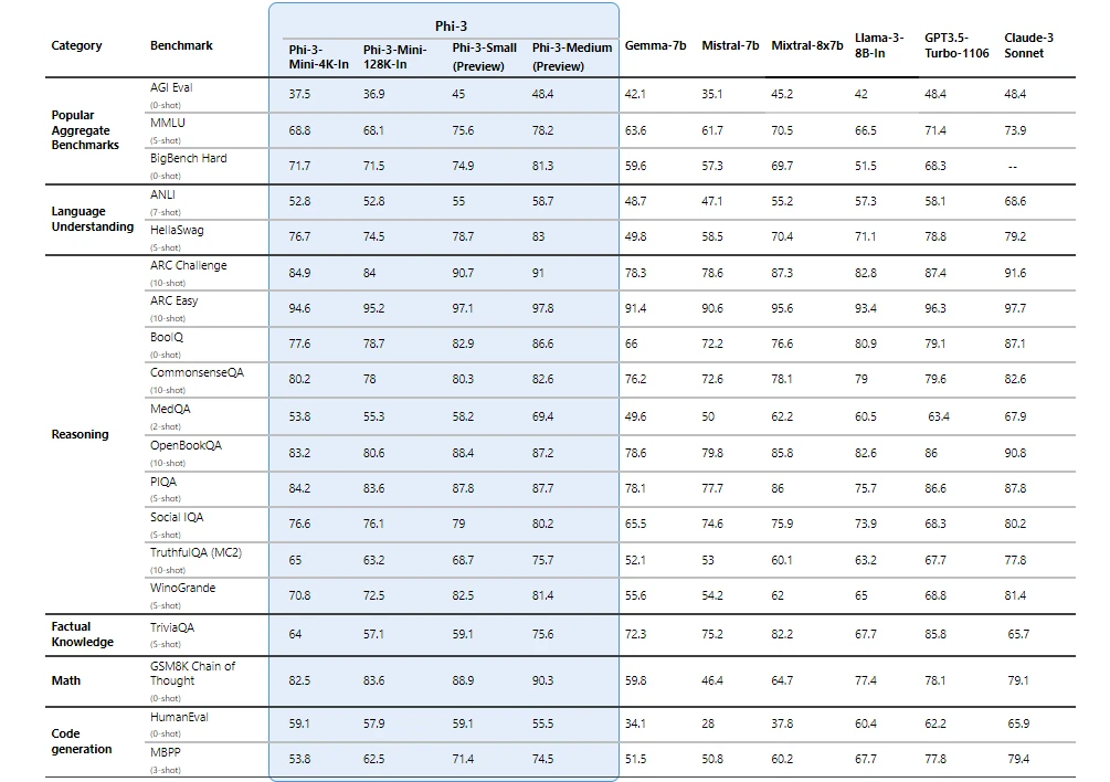
Phi-3 models significantly outperform language models of the same and larger sizes on key benchmarks (see benchmark numbers below, higher is better). Phi-3-mini does better than models twice its size, and Phi-3-small and Phi-3-medium outperform much larger models, including GPT-3.5T.  

All reported numbers are produced with the same pipeline to ensure that the numbers are comparable. As a result, these numbers may differ from other published numbers due to slight differences in the evaluation methodology. More details on benchmarks are provided in our technical paper . 

Note: Phi-3 models do not perform as well on factual knowledge benchmarks (such as TriviaQA) as the smaller model size results in less capacity to retain facts.  

Safety-first model design 

Responsible ai principles

Phi-3 models were developed in accordance with the Microsoft Responsible AI Standard , which is a company-wide set of requirements based on the following six principles: accountability, transparency, fairness, reliability and safety, privacy and security, and inclusiveness. Phi-3 models underwent rigorous safety measurement and evaluation, red-teaming, sensitive use review, and adherence to security guidance to help ensure that these models are responsibly developed, tested, and deployed in alignment with Microsoft’s standards and best practices.  

Building on our prior work with Phi models (“ Textbooks Are All You Need ”), Phi-3 models are also trained using high-quality data. They were further improved with extensive safety post-training, including reinforcement learning from human feedback (RLHF), automated testing and evaluations across dozens of harm categories, and manual red-teaming. Our approach to safety training and evaluations are detailed in our technical paper , and we outline recommended uses and limitations in the model cards. See the model card collection .  

Unlocking new capabilities 

Microsoft’s experience shipping copilots and enabling customers to transform their businesses with generative AI using Azure AI has highlighted the growing need for different-size models across the quality-cost curve for different tasks. Small language models, like Phi-3, are especially great for: 

• Resource constrained environments including on-device and offline inference scenarios.
• Latency bound scenarios where fast response times are critical.
• Cost constrained use cases, particularly those with simpler tasks.

For more on small language models, see our Microsoft Source Blog .

Thanks to their smaller size, Phi-3 models can be used in compute-limited inference environments. Phi-3-mini, in particular, can be used on-device, especially when further optimized with ONNX Runtime for cross-platform availability. The smaller size of Phi-3 models also makes fine-tuning or customization easier and more affordable. In addition, their lower computational needs make them a lower cost option with much better latency. The longer context window enables taking in and reasoning over large text content—documents, web pages, code, and more. Phi-3-mini demonstrates strong reasoning and logic capabilities, making it a good candidate for analytical tasks. 

Customers are already building solutions with Phi-3. One example where Phi-3 is already demonstrating value is in agriculture, where internet might not be readily accessible. Powerful small models like Phi-3 along with Microsoft copilot templates are available to farmers at the point of need and provide the additional benefit of running at reduced cost, making AI technologies even more accessible.  

ITC, a leading business conglomerate based in India, is leveraging Phi-3 as part of their continued collaboration with Microsoft on the copilot for Krishi Mitra, a farmer-facing app that reaches over a million farmers.

“ Our goal with the Krishi Mitra copilot is to improve efficiency while maintaining the accuracy of a large language model. We are excited to partner with Microsoft on using fine-tuned versions of Phi-3 to meet both our goals—efficiency and accuracy! ”    Saif Naik, Head of Technology, ITCMAARS

Originating in Microsoft Research, Phi models have been broadly used, with Phi-2 downloaded over 2 million times. The Phi series of models have achieved remarkable performance with strategic data curation and innovative scaling. Starting with Phi-1, a model used for Python coding, to Phi-1.5, enhancing reasoning and understanding, and then to Phi-2, a 2.7 billion-parameter model outperforming those up to 25 times its size in language comprehension. 1 Each iteration has leveraged high-quality training data and knowledge transfer techniques to challenge conventional scaling laws. 

Get started today 

To experience Phi-3 for yourself, start with playing with the model on Azure AI Playground . You can also find the model on the Hugging Chat playground . Start building with and customizing Phi-3 for your scenarios using the  Azure AI Studio . Join us to learn more about Phi-3 during a special  live stream of the AI Show.  

1 Microsoft Research Blog, Phi-2: The surprising power of small language models, December 12, 2023 .

Let us know what you think of Azure and what you would like to see in the future.

Provide feedback

Build your cloud computing and Azure skills with free courses by Microsoft Learn.

Explore Azure learning

Related posts

AI + Machine Learning , Azure AI , Azure AI Content Safety , Azure Cognitive Search , Azure Kubernetes Service (AKS) , Azure OpenAI Service , Customer stories

AI-powered dialogues: Global telecommunications with Azure OpenAI Service   chevron_right

AI + Machine Learning , Azure AI , Azure AI Content Safety , Azure OpenAI Service , Customer stories

Generative AI and the path to personalized medicine with Microsoft Azure   chevron_right

AI + Machine Learning , Azure AI , Azure AI Services , Azure AI Studio , Azure OpenAI Service , Best practices

AI study guide: The no-cost tools from Microsoft to jump start your generative AI journey   chevron_right

AI + Machine Learning , Azure AI , Azure VMware Solution , Events , Microsoft Copilot for Azure , Microsoft Defender for Cloud

Get ready for AI at the Migrate to Innovate digital event   chevron_right