hypothesis testing practice problems

9.4 Full Hypothesis Test Examples

Tests on means, example 9.8.

Jeffrey, as an eight-year old, established a mean time of 16.43 seconds for swimming the 25-yard freestyle, with a standard deviation of 0.8 seconds . His dad, Frank, thought that Jeffrey could swim the 25-yard freestyle faster using goggles. Frank bought Jeffrey a new pair of expensive goggles and timed Jeffrey for 15 25-yard freestyle swims . For the 15 swims, Jeffrey's mean time was 16 seconds. Frank thought that the goggles helped Jeffrey to swim faster than the 16.43 seconds. Conduct a hypothesis test using a preset α = 0.05. Assume that the swim times for the 25-yard freestyle are normal.

Set up the Hypothesis Test:

Since the problem is about a mean, this is a test of a single population mean .

H 0 : μ = 16.43   H a : μ < 16.43

For Jeffrey to swim faster, his time will be less than 16.43 seconds. The "<" tells you this is left-tailed.

Determine the distribution needed:

Random variable: X ¯ X ¯ = the mean time to swim the 25-yard freestyle.

Distribution for the test: X ¯ X ¯ is normal (population standard deviation is known: σ = 0.8)

X ¯ ~ N ( μ , σ X n ) X ¯ ~ N ( μ , σ X n ) Therefore, X ¯ ~ N ( 16.43 , 0.8 15 ) X ¯ ~ N ( 16.43 , 0.8 15 )

μ = 16.43 comes from H 0 and not the data. σ = 0.8, and n = 15.

Calculate the p -value using the normal distribution for a mean:

p -value = P ( x ¯ x ¯ < 16) = 0.0187 where the sample mean in the problem is given as 16.

p -value = 0.0187 (This is called the actual level of significance .) The p -value is the area to the left of the sample mean is given as 16.

μ = 16.43 comes from H 0 . Our assumption is μ = 16.43.

Interpretation of the p -value: If H 0 is true , there is a 0.0187 probability (1.87%)that Jeffrey's mean time to swim the 25-yard freestyle is 16 seconds or less. Because a 1.87% chance is small, the mean time of 16 seconds or less is unlikely to have happened randomly. It is a rare event.

Compare α and the p -value:

α = 0.05 p -value = 0.0187 α > p -value

Make a decision: Since α > α > p -value, reject H 0 .

This indicates that you reject the null hypothesis that the mean time to swim the 25-yard freestyle is at least 16.43 seconds.

Conclusion: At the 5% significance level, there is sufficient evidence that Jeffrey's mean time to swim the 25-yard freestyle is less than 16.43 seconds. Thus, based on the sample data, we conclude that Jeffrey swims faster using the new goggles.

The Type I and Type II errors for this problem are as follows: The Type I error is to conclude that Jeffrey swims the 25-yard freestyle, on average, in less than 16.43 seconds when, in fact, he actually swims the 25-yard freestyle, on average, in at least 16.43 seconds. (Reject the null hypothesis when the null hypothesis is true.)

The Type II error is that there is not evidence to conclude that Jeffrey swims the 25-yard freestyle, on average, in less than 16.43 seconds when, in fact, he actually does swim the 25-yard free-style, on average, in less than 16.43 seconds. (Do not reject the null hypothesis when the null hypothesis is false.)

The mean throwing distance of a football for Marco, a high school quarterback, is 40 yards, with a standard deviation of two yards. The team coach tells Marco to adjust his grip to get more distance. The coach records the distances for 20 throws. For the 20 throws, Marco’s mean distance was 45 yards. The coach thought the different grip helped Marco throw farther than 40 yards. Conduct a hypothesis test using a preset α = 0.05. Assume the throw distances for footballs are normal.

First, determine what type of test this is, set up the hypothesis test, find the p -value, sketch the graph, and state your conclusion.

Example 9.9

Jasmine has just begun her new job on the sales force of a very competitive company. In a sample of 16 sales calls it was found that she closed the contract for an average value of 108 dollars with a standard deviation of 12 dollars. Test at 5% significance that the population mean is at least 100 dollars against the alternative that it is less than 100 dollars. Company policy requires that new members of the sales force must exceed an average of $100 per contract during the trial employment period. Can we conclude that Jasmine has met this requirement at the significance level of 95%?

• H 0 : µ ≤ 100 H a : µ > 100 The null and alternative hypothesis are for the parameter µ because the number of dollars of the contracts is a continuous random variable. Also, this is a one-tailed test because the company has only an interested if the number of dollars per contact is below a particular number not "too high" a number. This can be thought of as making a claim that the requirement is being met and thus the claim is in the alternative hypothesis.
• Test statistic: t c = x ¯ − µ 0 s n = 108 − 100 ( 12 16 ) = 2.67 t c = x ¯ − µ 0 s n = 108 − 100 ( 12 16 ) = 2.67
• Critical value: t a = 1.753 t a = 1.753 with n-1 degrees of freedom= 15

The test statistic is a Student's t because the sample size is below 30; therefore, we cannot use the normal distribution. Comparing the calculated value of the test statistic and the critical value of t t ( t a ) ( t a ) at a 5% significance level, we see that the calculated value is in the tail of the distribution. Thus, we conclude that 108 dollars per contract is significantly larger than the hypothesized value of 100 and thus we cannot accept the null hypothesis. There is evidence that supports Jasmine's performance meets company standards.

It is believed that a stock price for a particular company will grow at a rate of $5 per week with a standard deviation of $1. An investor believes the stock won’t grow as quickly. The changes in stock price is recorded for ten weeks and are as follows: $4, $3, $2, $3, $1, $7, $2, $1, $1, $2. Perform a hypothesis test using a 5% level of significance. State the null and alternative hypotheses, state your conclusion, and identify the Type I errors.

Example 9.10

A manufacturer of salad dressings uses machines to dispense liquid ingredients into bottles that move along a filling line. The machine that dispenses salad dressings is working properly when 8 ounces are dispensed. Suppose that the average amount dispensed in a particular sample of 35 bottles is 7.91 ounces with a variance of 0.03 ounces squared, s 2 s 2 . Is there evidence that the machine should be stopped and production wait for repairs? The lost production from a shutdown is potentially so great that management feels that the level of significance in the analysis should be 99%.

Again we will follow the steps in our analysis of this problem.

STEP 1 : Set the Null and Alternative Hypothesis. The random variable is the quantity of fluid placed in the bottles. This is a continuous random variable and the parameter we are interested in is the mean. Our hypothesis therefore is about the mean. In this case we are concerned that the machine is not filling properly. From what we are told it does not matter if the machine is over-filling or under-filling, both seem to be an equally bad error. This tells us that this is a two-tailed test: if the machine is malfunctioning it will be shutdown regardless if it is from over-filling or under-filling. The null and alternative hypotheses are thus:

STEP 2 : Decide the level of significance and draw the graph showing the critical value.

This problem has already set the level of significance at 99%. The decision seems an appropriate one and shows the thought process when setting the significance level. Management wants to be very certain, as certain as probability will allow, that they are not shutting down a machine that is not in need of repair. To draw the distribution and the critical value, we need to know which distribution to use. Because this is a continuous random variable and we are interested in the mean, and the sample size is greater than 30, the appropriate distribution is the normal distribution and the relevant critical value is 2.575 from the normal table or the t-table at 0.005 column and infinite degrees of freedom. We draw the graph and mark these points.

STEP 3 : Calculate sample parameters and the test statistic. The sample parameters are provided, the sample mean is 7.91 and the sample variance is .03 and the sample size is 35. We need to note that the sample variance was provided not the sample standard deviation, which is what we need for the formula. Remembering that the standard deviation is simply the square root of the variance, we therefore know the sample standard deviation, s, is 0.173. With this information we calculate the test statistic as -3.07, and mark it on the graph.

STEP 4 : Compare test statistic and the critical values Now we compare the test statistic and the critical value by placing the test statistic on the graph. We see that the test statistic is in the tail, decidedly greater than the critical value of 2.575. We note that even the very small difference between the hypothesized value and the sample value is still a large number of standard deviations. The sample mean is only 0.08 ounces different from the required level of 8 ounces, but it is 3 plus standard deviations away and thus we cannot accept the null hypothesis.

STEP 5 : Reach a Conclusion

Three standard deviations of a test statistic will guarantee that the test will fail. The probability that anything is within three standard deviations is almost zero. Actually it is 0.0026 on the normal distribution, which is certainly almost zero in a practical sense. Our formal conclusion would be “ At a 99% level of significance we cannot accept the hypothesis that the sample mean came from a distribution with a mean of 8 ounces” Or less formally, and getting to the point, “At a 99% level of significance we conclude that the machine is under filling the bottles and is in need of repair”.

Try It 9.10

A company records the mean time of employees working in a day. The mean comes out to be 475 minutes, with a standard deviation of 45 minutes. A manager recorded times of 20 employees. The times of working were (frequencies are in parentheses) 460(3); 465(2); 470(3); 475(1); 480(6); 485(3); 490(2).

Conduct a hypothesis test using a 2.5% level of significance to determine if the mean time is more than 475 .

Hypothesis Test for Proportions

Just as there were confidence intervals for proportions, or more formally, the population parameter p of the binomial distribution, there is the ability to test hypotheses concerning p .

The population parameter for the binomial is p . The estimated value (point estimate) for p is p′ where p′ = x/n , x is the number of successes in the sample and n is the sample size.

When you perform a hypothesis test of a population proportion p , you take a simple random sample from the population. The conditions for a binomial distribution must be met, which are: there are a certain number n of independent trials meaning random sampling, the outcomes of any trial are binary, success or failure, and each trial has the same probability of a success p . The shape of the binomial distribution needs to be similar to the shape of the normal distribution. To ensure this, the quantities np′ and nq′ must both be greater than five ( np′ > 5 and nq′ > 5). In this case the binomial distribution of a sample (estimated) proportion can be approximated by the normal distribution with μ = np μ = np and σ = npq σ = npq . Remember that q = 1 – p q = 1 – p . There is no distribution that can correct for this small sample bias and thus if these conditions are not met we simply cannot test the hypothesis with the data available at that time. We met this condition when we first were estimating confidence intervals for p .

Again, we begin with the standardizing formula modified because this is the distribution of a binomial.

Substituting p 0 p 0 , the hypothesized value of p , we have:

This is the test statistic for testing hypothesized values of p , where the null and alternative hypotheses take one of the following forms:

The decision rule stated above applies here also: if the calculated value of Z c shows that the sample proportion is "too many" standard deviations from the hypothesized proportion, the null hypothesis cannot be accepted. The decision as to what is "too many" is pre-determined by the analyst depending on the level of significance required in the test.

Example 9.11

The mortgage department of a large bank is interested in the nature of loans of first-time borrowers. This information will be used to tailor their marketing strategy. They believe that 50% of first-time borrowers take out smaller loans than other borrowers. They perform a hypothesis test to determine if the percentage is the same or different from 50% . They sample 100 first-time borrowers and find 53 of these loans are smaller that the other borrowers. For the hypothesis test, they choose a 5% level of significance.

STEP 1 : Set the null and alternative hypothesis.

H 0 : p = 0.50   H a : p ≠ 0.50

The words "is the same or different from" tell you this is a two-tailed test. The Type I and Type II errors are as follows: The Type I error is to conclude that the proportion of borrowers is different from 50% when, in fact, the proportion is actually 50%. (Reject the null hypothesis when the null hypothesis is true). The Type II error is there is not enough evidence to conclude that the proportion of first time borrowers differs from 50% when, in fact, the proportion does differ from 50%. (You fail to reject the null hypothesis when the null hypothesis is false.)

STEP 2 : Decide the level of significance and draw the graph showing the critical value

The level of significance has been set by the problem at the 5% level. Because this is two-tailed test one-half of the alpha value will be in the upper tail and one-half in the lower tail as shown on the graph. The critical value for the normal distribution at the 95% level of confidence is 1.96. This can easily be found on the student’s t-table at the very bottom at infinite degrees of freedom remembering that at infinity the t-distribution is the normal distribution. Of course the value can also be found on the normal table but you have go looking for one-half of 95 (0.475) inside the body of the table and then read out to the sides and top for the number of standard deviations.

STEP 3 : Calculate the sample parameters and critical value of the test statistic.

The test statistic is a normal distribution, Z, for testing proportions and is:

For this case, the sample of 100 found 53 of these loans were smaller than those of other borrowers. The sample proportion, p′ = 53/100= 0.53 The test question, therefore, is : “Is 0.53 significantly different from .50?” Putting these values into the formula for the test statistic we find that 0.53 is only 0.60 standard deviations away from .50. This is barely off of the mean of the standard normal distribution of zero. There is virtually no difference from the sample proportion and the hypothesized proportion in terms of standard deviations.

STEP 4 : Compare the test statistic and the critical value.

The calculated value is well within the critical values of ± 1.96 standard deviations and thus we cannot reject the null hypothesis. To reject the null hypothesis we need significant evident of difference between the hypothesized value and the sample value. In this case the sample value is very nearly the same as the hypothesized value measured in terms of standard deviations.

STEP 5 : Reach a conclusion

The formal conclusion would be “At a 5% level of significance we cannot reject the null hypothesis that 50% of first-time borrowers take out smaller loans than other borrowers.” Notice the length to which the conclusion goes to include all of the conditions that are attached to the conclusion. Statisticians, for all the criticism they receive, are careful to be very specific even when this seems trivial. Statisticians cannot say more than they know, and the data constrain the conclusion to be within the metes and bounds of the data.

Try It 9.11

A teacher believes that 85% of students in the class will want to go on a field trip to the local zoo. The teacher performs a hypothesis test to determine if the percentage is the same or different from 85%. The teacher samples 50 students and 39 reply that they would want to go to the zoo. For the hypothesis test, use a 1% level of significance.

Example 9.12

Suppose a consumer group suspects that the proportion of households that have three or more cell phones is 30%. A cell phone company has reason to believe that the proportion is not 30%. Before they start a big advertising campaign, they conduct a hypothesis test. Their marketing people survey 150 households with the result that 43 of the households have three or more cell phones.

Here is an abbreviate version of the system to solve hypothesis tests applied to a test on a proportions.

Try It 9.12

Marketers believe that 92% of adults in the United States own a cell phone. A cell phone manufacturer believes that number is actually lower. 200 American adults are surveyed, of which, 174 report having cell phones. Use a 5% level of significance. State the null and alternative hypothesis, find the p -value, state your conclusion, and identify the Type I and Type II errors.

Example 9.13

The National Institute of Standards and Technology provides exact data on conductivity properties of materials. Following are conductivity measurements for 11 randomly selected pieces of a particular type of glass.

1.11; 1.07; 1.11; 1.07; 1.12; 1.08; .98; .98; 1.02; .95; .95 Is there convincing evidence that the average conductivity of this type of glass is greater than one? Use a significance level of 0.05.

Let’s follow a four-step process to answer this statistical question.

• H 0 : μ ≤ 1
• H a : μ > 1
• Plan : We are testing a sample mean without a known population standard deviation with less than 30 observations. Therefore, we need to use a Student's-t distribution. Assume the underlying population is normal.
• Do the calculations and draw the graph .
• State the Conclusions : We cannot accept the null hypothesis. It is reasonable to state that the data supports the claim that the average conductivity level is greater than one.

Try It 9.13

The boiling point of a specific liquid is measured for 15 samples, and the boiling points are obtained as follows:

205; 206; 206; 202; 199; 194; 197; 198; 198; 201; 201; 202; 207; 211; 205

Is there convincing evidence that the average boiling point is greater than 200? Use a significance level of 0.1. Assume the population is normal.

Example 9.14

In a study of 420,019 cell phone users, 172 of the subjects developed brain cancer. Test the claim that cell phone users developed brain cancer at a greater rate than that for non-cell phone users (the rate of brain cancer for non-cell phone users is 0.0340%). Since this is a critical issue, use a 0.005 significance level. Explain why the significance level should be so low in terms of a Type I error.

• H 0 : p ≤ 0.00034
• H a : p > 0.00034

If we commit a Type I error, we are essentially accepting a false claim. Since the claim describes cancer-causing environments, we want to minimize the chances of incorrectly identifying causes of cancer.

• We will be testing a sample proportion with x = 172 and n = 420,019. The sample is sufficiently large because we have np' = 420,019(0.00034) = 142.8, nq' = 420,019(0.99966) = 419,876.2, two independent outcomes, and a fixed probability of success p' = 0.00034. Thus we will be able to generalize our results to the population.

Try It 9.14

In a study of 390,000 moisturizer users, 138 of the subjects developed skin diseases. Test the claim that moisturizer users developed skin diseases at a greater rate than that for non-moisturizer users (the rate of skin diseases for non-moisturizer users is 0.041%). Since this is a critical issue, use a 0.005 significance level. Explain why the significance level should be so low in terms of a Type I error.

This book may not be used in the training of large language models or otherwise be ingested into large language models or generative AI offerings without OpenStax's permission.

Want to cite, share, or modify this book? This book uses the Creative Commons Attribution License and you must attribute OpenStax.

Access for free at https://openstax.org/books/introductory-business-statistics-2e/pages/1-introduction

• Authors: Alexander Holmes, Barbara Illowsky, Susan Dean
• Publisher/website: OpenStax
• Book title: Introductory Business Statistics 2e
• Publication date: Dec 13, 2023
• Location: Houston, Texas
• Book URL: https://openstax.org/books/introductory-business-statistics-2e/pages/1-introduction
• Section URL: https://openstax.org/books/introductory-business-statistics-2e/pages/9-4-full-hypothesis-test-examples

© Dec 6, 2023 OpenStax. Textbook content produced by OpenStax is licensed under a Creative Commons Attribution License . The OpenStax name, OpenStax logo, OpenStax book covers, OpenStax CNX name, and OpenStax CNX logo are not subject to the Creative Commons license and may not be reproduced without the prior and express written consent of Rice University.

• Number Theory
• Data Structures
• Cornerstones

Exercises - Hypothesis Tests for Proportions (Two Samples)

A researcher wants to examine the possibility that women are more likely to commit suicide off a cliff than men are. Data from the past 5 years show that out of 987 men who committed suicide, 394 jumped off a cliff. On the other hand, $44\%$ of the 500 women who committed suicide did so by jumping off a cliff.

What can be said about the researcher's claim? Use the $P$-value method with a significance level of $\alpha=0.05$.

A survey asks a random sample of men and women whether they agree with a particular statement. The result of the survey is that $35\%$ of the men and $43\%$ of the women agree with the statement. The maximum error of the estimate for the difference in proportions is calculated to be 0.135.

• Find the confidence interval for the difference in the proportions of men and women who agree.
• Should we reject the null hypothesis $p_M=p_W$? Explain.
• $-.215 \lt p_M-p_W \lt .055$
• Fail to reject the null hypothesis because 0 is in the confidence interval.
• Find a $95\%$ confidence interval for the difference in the proportions of satisfied freshmen and sophomores.
• Using the confidence interval above, test the claim that there is no difference in the proportion of satisfied freshmen and sophomores. (Use $ \alpha=.05$.)

Assumptions: $29,\ 11,\ 23,\ 17 \geq 5$; $E=.206$ Confidence interval: $-.056 \lt p_F-p_S \lt .356$ Interpretation: We are $95\%$ confident that the difference in the proportions of satisfied freshmen and sophomores is between -.056 and .356.

• The null hypothesis for testing this claim would be $H_0 : p_F - p_S = 0$. As this $0$ is in the confidence interval (as expected), we fail to reject the null hypothesis. There is no evidence of a difference in the proportions of satisfied freshmen and sophomores.

Data Science Duniya

Learn Data Science, Machine Learning and Artificial Intelligence

Practice Problems on Hypothesis Testing

In this post I have put together the practice problems (from my academics study notes) to explain how in practical Hypothesis Testing works. This post is written mostly for the learners who want to deep dive into the statistics for data science. Focus will be on problem solving. For concepts please refer my previous posts on testing of hypothesis.

Prerequisite to understand Hypothesis testing examples:

• Understanding of hypothesis testing concepts
• How to use z-table, t-table and chi square table.

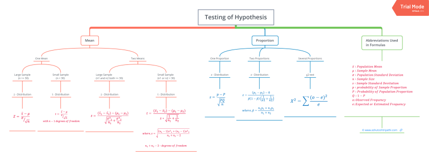
Formula list:

Critical Regions

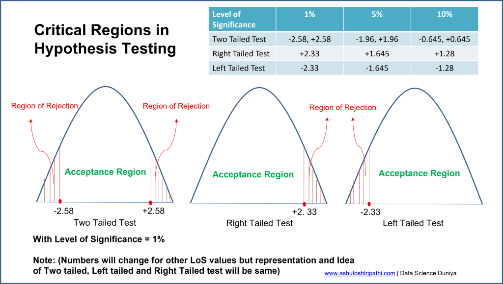
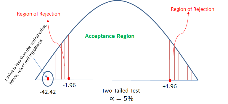
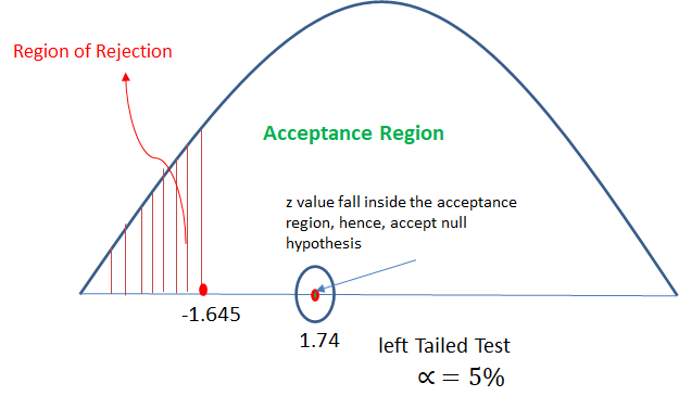
In hypothesis testing, critical region is represented by set of values, where null hypothesis is rejected. So it is also know as region of rejection. It takes different boundary values for different level of significance. Below info graphics shows the region of rejection that is critical region and region of acceptance with respect to the level of significance 1%.

A Telecom service provider claims that individual customers pay on an average 400 rs. per month with standard deviation of 25 rs. A random sample of 50 customers bills during a given month is taken with a mean of 250 and standard deviation of 15. What to say with respect to the claim made by the service provider?

From the data available, it is observed that 400 out of 850 customers purchased the groceries online. Can we say that most of the customers are moving towards online shopping even for groceries?

It is found that 250 errors in the randomly selected 1000 lines of code from Team A and 300 errors in 800 lines of code from Team B. Can we assume that team B’s performance is superior to that of A.

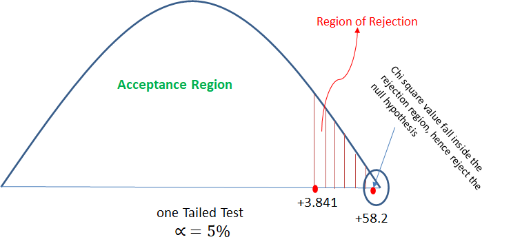
Following is the record of number of accidents took place during the various days of the week.

Can we conclude that accident s are independent of the day of week?

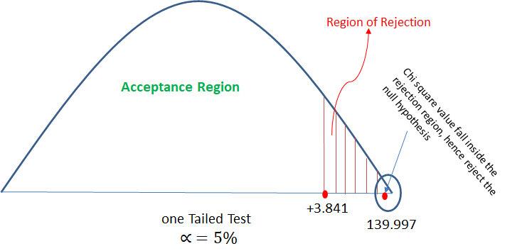
Analyze the below data and tell whether you can conclude that smoking causes cancer or not?

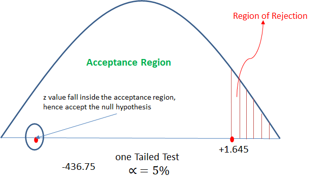
It is claimed that the mean of the population is 67 at 5% level of significance. Mean obtained from a random sample of size 100 is 64 with SD 3. Validate the claim.

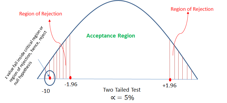
There is an assumption that there is no significant difference between boys and girls with respect to intelligence. Tests are conducted on two groups and the following are the observations

Validate the claim with 5% LoS (Level of Significance)

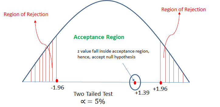
An automobile tyre manufacturer claims that the average life of a particular grade of tyre is more than 20,000 km. A random sample of 16 tyres is having mean 22,000 km with a standard deviation of 5000 km.

Validate the claim of the manufacturer at 5% LoS.

That is all for now. Please share your thoughts using the comment section below.

Type your email…

Share this:

• Click to share on Twitter (Opens in new window)
• Click to share on Facebook (Opens in new window)
• Click to print (Opens in new window)
• Click to email a link to a friend (Opens in new window)
• Click to share on LinkedIn (Opens in new window)
• Click to share on Reddit (Opens in new window)
• Click to share on WhatsApp (Opens in new window)
• Click to share on Tumblr (Opens in new window)
• Click to share on Pinterest (Opens in new window)
• Click to share on Pocket (Opens in new window)
• Click to share on Telegram (Opens in new window)

I think smoking problem is wrongly concluded. There the H0 is assumed of dependency(smoking and cancer are dependent) while for chi square test, the null hypothesis is always for independence. So the H0 should be “Smoking and Cancer are independent”.

Please how can I download this page?

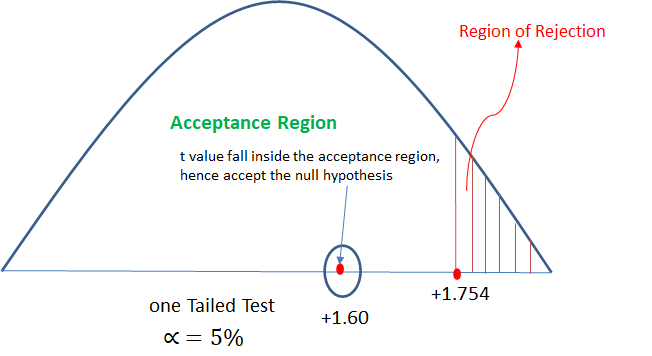
In the last sum the alternate hypothesis is less than 22,000 and the null hypothesis is more than 20,000. If the value turns out to be 21,000 then which hypothesis will you accept? I guess there’s an error, the alternate hypothesis should be less than equal to 20,000 and not 22,000. Correct me if I’m wrong.

Thanks for presenting above test cases, it really really helps to understand the tail concept. I am reading z-test and refer your hypothesis page as an example. I go through z-test example and in example no.8 last one it is “One tail – Left tailed test” but in the diag below it shows the right tailed. Not sure am I interpret wrong or diag error ? pls . correct me. Thanks.

The alternate hypothesis is the opposite of null hypothesis so it’s less less than or left tailed. Since the null hypothesis was accepted the graph is Right Tailed had the null hypothesis been rejected or the alternate hypothesis been accepted the graph would have been left tailed. I hope I cleared your doubt

Leave a Reply Cancel reply

This site uses Akismet to reduce spam. Learn how your comment data is processed .

• Already have a WordPress.com account? Log in now.
• Subscribe Subscribed
• Copy shortlink
• Report this content
• View post in Reader
• Manage subscriptions
• Collapse this bar

User Preferences

Content preview.

Arcu felis bibendum ut tristique et egestas quis:

• Ut enim ad minim veniam, quis nostrud exercitation ullamco laboris
• Duis aute irure dolor in reprehenderit in voluptate
• Excepteur sint occaecat cupidatat non proident

Keyboard Shortcuts

S.3.2 hypothesis testing (p-value approach).

The P -value approach involves determining "likely" or "unlikely" by determining the probability — assuming the null hypothesis was true — of observing a more extreme test statistic in the direction of the alternative hypothesis than the one observed. If the P -value is small, say less than (or equal to) \(\alpha\), then it is "unlikely." And, if the P -value is large, say more than \(\alpha\), then it is "likely."

If the P -value is less than (or equal to) \(\alpha\), then the null hypothesis is rejected in favor of the alternative hypothesis. And, if the P -value is greater than \(\alpha\), then the null hypothesis is not rejected.

Specifically, the four steps involved in using the P -value approach to conducting any hypothesis test are:

• Specify the null and alternative hypotheses.
• Using the sample data and assuming the null hypothesis is true, calculate the value of the test statistic. Again, to conduct the hypothesis test for the population mean μ , we use the t -statistic \(t^*=\frac{\bar{x}-\mu}{s/\sqrt{n}}\) which follows a t -distribution with n - 1 degrees of freedom.
• Using the known distribution of the test statistic, calculate the P -value : "If the null hypothesis is true, what is the probability that we'd observe a more extreme test statistic in the direction of the alternative hypothesis than we did?" (Note how this question is equivalent to the question answered in criminal trials: "If the defendant is innocent, what is the chance that we'd observe such extreme criminal evidence?")
• Set the significance level, \(\alpha\), the probability of making a Type I error to be small — 0.01, 0.05, or 0.10. Compare the P -value to \(\alpha\). If the P -value is less than (or equal to) \(\alpha\), reject the null hypothesis in favor of the alternative hypothesis. If the P -value is greater than \(\alpha\), do not reject the null hypothesis.

Example S.3.2.1

Mean gpa section  .

In our example concerning the mean grade point average, suppose that our random sample of n = 15 students majoring in mathematics yields a test statistic t * equaling 2.5. Since n = 15, our test statistic t * has n - 1 = 14 degrees of freedom. Also, suppose we set our significance level α at 0.05 so that we have only a 5% chance of making a Type I error.

Right Tailed

The P -value for conducting the right-tailed test H 0 : μ = 3 versus H A : μ > 3 is the probability that we would observe a test statistic greater than t * = 2.5 if the population mean \(\mu\) really were 3. Recall that probability equals the area under the probability curve. The P -value is therefore the area under a t n - 1 = t 14 curve and to the right of the test statistic t * = 2.5. It can be shown using statistical software that the P -value is 0.0127. The graph depicts this visually.

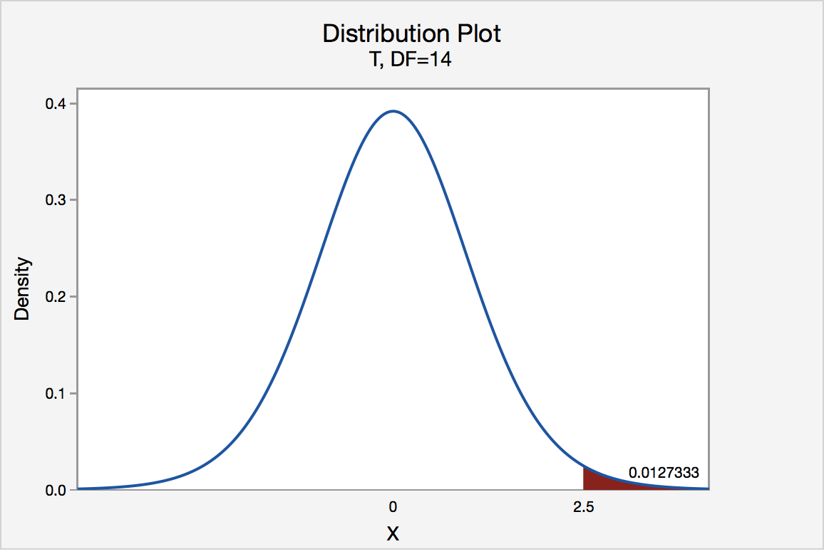
The P -value, 0.0127, tells us it is "unlikely" that we would observe such an extreme test statistic t * in the direction of H A if the null hypothesis were true. Therefore, our initial assumption that the null hypothesis is true must be incorrect. That is, since the P -value, 0.0127, is less than \(\alpha\) = 0.05, we reject the null hypothesis H 0 : μ = 3 in favor of the alternative hypothesis H A : μ > 3.

Note that we would not reject H 0 : μ = 3 in favor of H A : μ > 3 if we lowered our willingness to make a Type I error to \(\alpha\) = 0.01 instead, as the P -value, 0.0127, is then greater than \(\alpha\) = 0.01.

Left Tailed

In our example concerning the mean grade point average, suppose that our random sample of n = 15 students majoring in mathematics yields a test statistic t * instead of equaling -2.5. The P -value for conducting the left-tailed test H 0 : μ = 3 versus H A : μ < 3 is the probability that we would observe a test statistic less than t * = -2.5 if the population mean μ really were 3. The P -value is therefore the area under a t n - 1 = t 14 curve and to the left of the test statistic t* = -2.5. It can be shown using statistical software that the P -value is 0.0127. The graph depicts this visually.

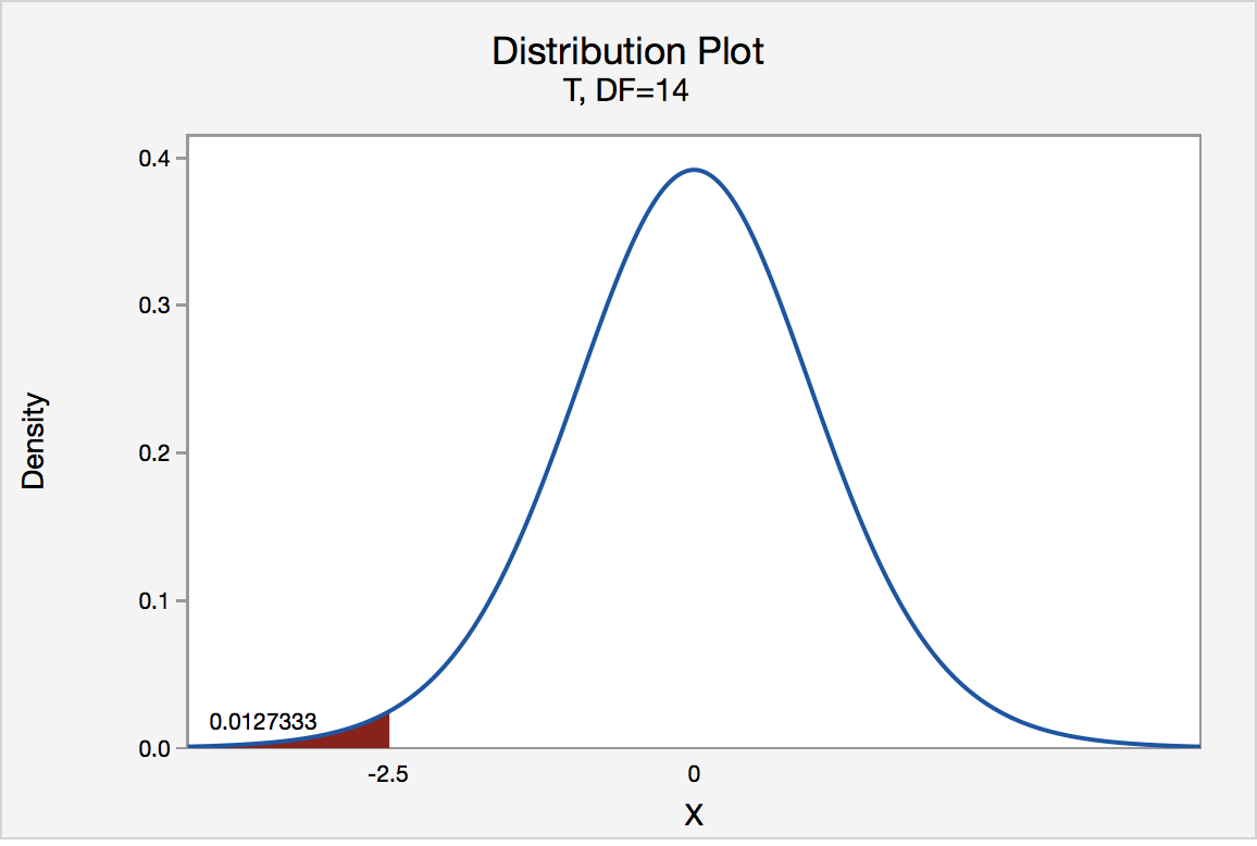
The P -value, 0.0127, tells us it is "unlikely" that we would observe such an extreme test statistic t * in the direction of H A if the null hypothesis were true. Therefore, our initial assumption that the null hypothesis is true must be incorrect. That is, since the P -value, 0.0127, is less than α = 0.05, we reject the null hypothesis H 0 : μ = 3 in favor of the alternative hypothesis H A : μ < 3.

Note that we would not reject H 0 : μ = 3 in favor of H A : μ < 3 if we lowered our willingness to make a Type I error to α = 0.01 instead, as the P -value, 0.0127, is then greater than \(\alpha\) = 0.01.

In our example concerning the mean grade point average, suppose again that our random sample of n = 15 students majoring in mathematics yields a test statistic t * instead of equaling -2.5. The P -value for conducting the two-tailed test H 0 : μ = 3 versus H A : μ ≠ 3 is the probability that we would observe a test statistic less than -2.5 or greater than 2.5 if the population mean μ really was 3. That is, the two-tailed test requires taking into account the possibility that the test statistic could fall into either tail (hence the name "two-tailed" test). The P -value is, therefore, the area under a t n - 1 = t 14 curve to the left of -2.5 and to the right of 2.5. It can be shown using statistical software that the P -value is 0.0127 + 0.0127, or 0.0254. The graph depicts this visually.

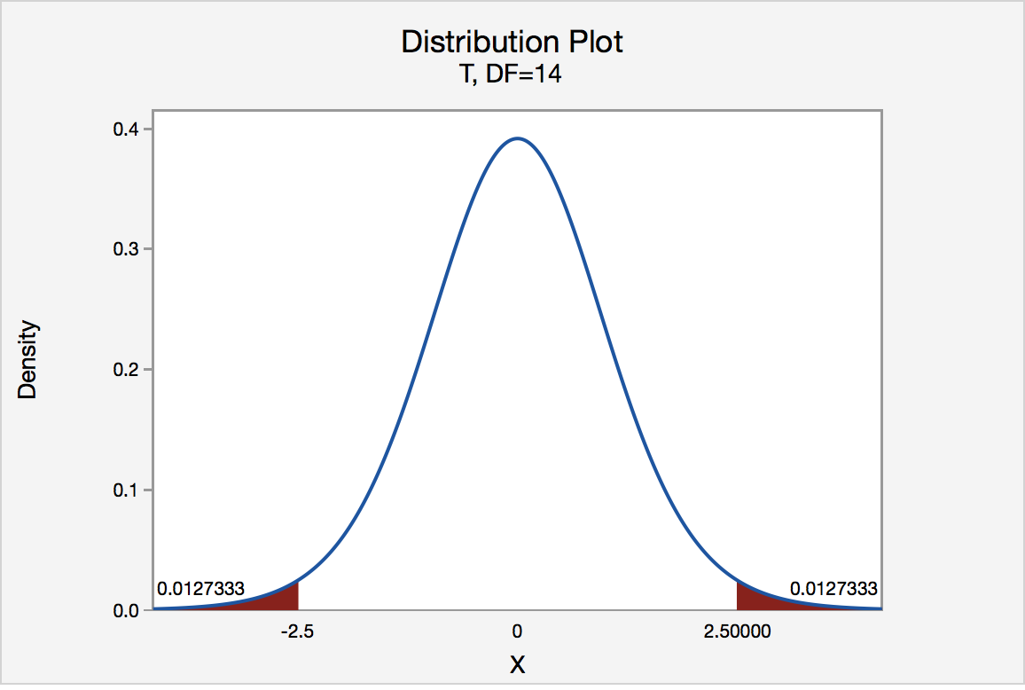
Note that the P -value for a two-tailed test is always two times the P -value for either of the one-tailed tests. The P -value, 0.0254, tells us it is "unlikely" that we would observe such an extreme test statistic t * in the direction of H A if the null hypothesis were true. Therefore, our initial assumption that the null hypothesis is true must be incorrect. That is, since the P -value, 0.0254, is less than α = 0.05, we reject the null hypothesis H 0 : μ = 3 in favor of the alternative hypothesis H A : μ ≠ 3.

Note that we would not reject H 0 : μ = 3 in favor of H A : μ ≠ 3 if we lowered our willingness to make a Type I error to α = 0.01 instead, as the P -value, 0.0254, is then greater than \(\alpha\) = 0.01.

Now that we have reviewed the critical value and P -value approach procedures for each of the three possible hypotheses, let's look at three new examples — one of a right-tailed test, one of a left-tailed test, and one of a two-tailed test.

The good news is that, whenever possible, we will take advantage of the test statistics and P -values reported in statistical software, such as Minitab, to conduct our hypothesis tests in this course.

• school Campus Bookshelves
• menu_book Bookshelves
• perm_media Learning Objects
• login Login
• how_to_reg Request Instructor Account
• hub Instructor Commons

Margin Size

• Download Page (PDF)
• Download Full Book (PDF)
• Periodic Table
• Physics Constants
• Scientific Calculator
• Reference & Cite
• Tools expand_more
• Readability

selected template will load here

This action is not available.

8.4: Hypothesis Test Examples for Proportions

• Last updated
• Save as PDF
• Page ID 11533

\( \newcommand{\vecs}[1]{\overset { \scriptstyle \rightharpoonup} {\mathbf{#1}} } \)

\( \newcommand{\vecd}[1]{\overset{-\!-\!\rightharpoonup}{\vphantom{a}\smash {#1}}} \)

\( \newcommand{\id}{\mathrm{id}}\) \( \newcommand{\Span}{\mathrm{span}}\)

( \newcommand{\kernel}{\mathrm{null}\,}\) \( \newcommand{\range}{\mathrm{range}\,}\)

\( \newcommand{\RealPart}{\mathrm{Re}}\) \( \newcommand{\ImaginaryPart}{\mathrm{Im}}\)

\( \newcommand{\Argument}{\mathrm{Arg}}\) \( \newcommand{\norm}[1]{\| #1 \|}\)

\( \newcommand{\inner}[2]{\langle #1, #2 \rangle}\)

\( \newcommand{\Span}{\mathrm{span}}\)

\( \newcommand{\id}{\mathrm{id}}\)

\( \newcommand{\kernel}{\mathrm{null}\,}\)

\( \newcommand{\range}{\mathrm{range}\,}\)

\( \newcommand{\RealPart}{\mathrm{Re}}\)

\( \newcommand{\ImaginaryPart}{\mathrm{Im}}\)

\( \newcommand{\Argument}{\mathrm{Arg}}\)

\( \newcommand{\norm}[1]{\| #1 \|}\)

\( \newcommand{\Span}{\mathrm{span}}\) \( \newcommand{\AA}{\unicode[.8,0]{x212B}}\)

\( \newcommand{\vectorA}[1]{\vec{#1}}      % arrow\)

\( \newcommand{\vectorAt}[1]{\vec{\text{#1}}}      % arrow\)

\( \newcommand{\vectorB}[1]{\overset { \scriptstyle \rightharpoonup} {\mathbf{#1}} } \)

\( \newcommand{\vectorC}[1]{\textbf{#1}} \)

\( \newcommand{\vectorD}[1]{\overrightarrow{#1}} \)

\( \newcommand{\vectorDt}[1]{\overrightarrow{\text{#1}}} \)

\( \newcommand{\vectE}[1]{\overset{-\!-\!\rightharpoonup}{\vphantom{a}\smash{\mathbf {#1}}}} \)

• In a hypothesis test problem, you may see words such as "the level of significance is 1%." The "1%" is the preconceived or preset \(\alpha\).
• The statistician setting up the hypothesis test selects the value of α to use before collecting the sample data.
• If no level of significance is given, a common standard to use is \(\alpha = 0.05\).
• When you calculate the \(p\)-value and draw the picture, the \(p\)-value is the area in the left tail, the right tail, or split evenly between the two tails. For this reason, we call the hypothesis test left, right, or two tailed.
• The alternative hypothesis, \(H_{a}\), tells you if the test is left, right, or two-tailed. It is the key to conducting the appropriate test.
• \(H_{a}\) never has a symbol that contains an equal sign.
• Thinking about the meaning of the \(p\)-value: A data analyst (and anyone else) should have more confidence that he made the correct decision to reject the null hypothesis with a smaller \(p\)-value (for example, 0.001 as opposed to 0.04) even if using the 0.05 level for alpha. Similarly, for a large p -value such as 0.4, as opposed to a \(p\)-value of 0.056 (\(\alpha = 0.05\) is less than either number), a data analyst should have more confidence that she made the correct decision in not rejecting the null hypothesis. This makes the data analyst use judgment rather than mindlessly applying rules.

Full Hypothesis Test Examples

Example \(\PageIndex{7}\)

Joon believes that 50% of first-time brides in the United States are younger than their grooms. She performs a hypothesis test to determine if the percentage is the same or different from 50% . Joon samples 100 first-time brides and 53 reply that they are younger than their grooms. For the hypothesis test, she uses a 1% level of significance.

Set up the hypothesis test:

The 1% level of significance means that α = 0.01. This is a test of a single population proportion .

\(H_{0}: p = 0.50\)  \(H_{a}: p \neq 0.50\)

The words "is the same or different from" tell you this is a two-tailed test.

Calculate the distribution needed:

Random variable: \(P′ =\) the percent of of first-time brides who are younger than their grooms.

Distribution for the test: The problem contains no mention of a mean. The information is given in terms of percentages. Use the distribution for P′ , the estimated proportion.

\[P' - N\left(p, \sqrt{\frac{p-q}{n}}\right)\nonumber \]

\[P' - N\left(0.5, \sqrt{\frac{0.5-0.5}{100}}\right)\nonumber \]

where \(p = 0.50, q = 1−p = 0.50\), and \(n = 100\)

Calculate the p -value using the normal distribution for proportions:

\[p\text{-value} = P(p′ < 0.47 or p′ > 0.53) = 0.5485\nonumber \]

where \[x = 53, p' = \frac{x}{n} = \frac{53}{100} = 0.53\nonumber \].

Interpretation of the \(p\text{-value})\: If the null hypothesis is true, there is 0.5485 probability (54.85%) that the sample (estimated) proportion \(p'\) is 0.53 or more OR 0.47 or less (see the graph in Figure).

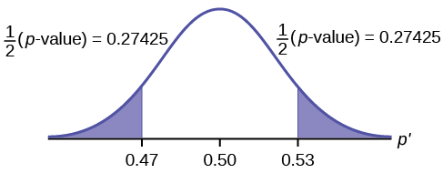
\(\mu = p = 0.50\) comes from \(H_{0}\), the null hypothesis.

\(p′ = 0.53\). Since the curve is symmetrical and the test is two-tailed, the \(p′\) for the left tail is equal to \(0.50 – 0.03 = 0.47\) where \(\mu = p = 0.50\). (0.03 is the difference between 0.53 and 0.50.)

Compare \(\alpha\) and the \(p\text{-value}\):

Since \(\alpha = 0.01\) and \(p\text{-value} = 0.5485\). \(\alpha < p\text{-value}\).

Make a decision: Since \(\alpha < p\text{-value}\), you cannot reject \(H_{0}\).

Conclusion: At the 1% level of significance, the sample data do not show sufficient evidence that the percentage of first-time brides who are younger than their grooms is different from 50%.

The \(p\text{-value}\) can easily be calculated.

Press STAT and arrow over to TESTS . Press 5:1-PropZTest . Enter .5 for \(p_{0}\), 53 for \(x\) and 100 for \(n\). Arrow down to Prop and arrow to not equals \(p_{0}\). Press ENTER . Arrow down to Calculate and press ENTER . The calculator calculates the \(p\text{-value}\) (\(p = 0.5485\)) and the test statistic (\(z\)-score). Prop not equals .5 is the alternate hypothesis. Do this set of instructions again except arrow to Draw (instead of Calculate ). Press ENTER . A shaded graph appears with \(\(z\) = 0.6\) (test statistic) and \(p = 0.5485\) (\(p\text{-value}\)). Make sure when you use Draw that no other equations are highlighted in \(Y =\) and the plots are turned off.

The Type I and Type II errors are as follows:

The Type I error is to conclude that the proportion of first-time brides who are younger than their grooms is different from 50% when, in fact, the proportion is actually 50%. (Reject the null hypothesis when the null hypothesis is true).

The Type II error is there is not enough evidence to conclude that the proportion of first time brides who are younger than their grooms differs from 50% when, in fact, the proportion does differ from 50%. (Do not reject the null hypothesis when the null hypothesis is false.)

Exercise \(\PageIndex{7}\)

A teacher believes that 85% of students in the class will want to go on a field trip to the local zoo. She performs a hypothesis test to determine if the percentage is the same or different from 85%. The teacher samples 50 students and 39 reply that they would want to go to the zoo. For the hypothesis test, use a 1% level of significance.

First, determine what type of test this is, set up the hypothesis test, find the \(p\text{-value}\), sketch the graph, and state your conclusion.

Since the problem is about percentages, this is a test of single population proportions.

• \(H_{0} : p = 0.85\)
• \(H_{a}: p \neq 0.85\)
• \(p = 0.7554\)

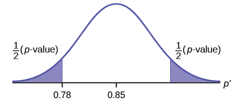
Because \(p > \alpha\), we fail to reject the null hypothesis. There is not sufficient evidence to suggest that the proportion of students that want to go to the zoo is not 85%.

Example \(\PageIndex{8}\)

Suppose a consumer group suspects that the proportion of households that have three cell phones is 30%. A cell phone company has reason to believe that the proportion is not 30%. Before they start a big advertising campaign, they conduct a hypothesis test. Their marketing people survey 150 households with the result that 43 of the households have three cell phones.

Set up the Hypothesis Test:

\(H_{0}: p = 0.30, H_{a}: p \neq 0.30\)

Determine the distribution needed:

The random variable is \(P′ =\) proportion of households that have three cell phones.

The distribution for the hypothesis test is \(P' - N\left(0.30, \sqrt{\frac{(0.30 \cdot 0.70)}{150}}\right)\)

Exercise 9.6.8.2

a. The value that helps determine the \(p\text{-value}\) is \(p′\). Calculate \(p′\).

a. \(p' = \frac{x}{n}\) where \(x\) is the number of successes and \(n\) is the total number in the sample.

\(x = 43, n = 150\)

\(p′ = 43150\)

Exercise 9.6.8.3

b. What is a success for this problem?

b. A success is having three cell phones in a household.

Exercise 9.6.8.4

c. What is the level of significance?

c. The level of significance is the preset \(\alpha\). Since \(\alpha\) is not given, assume that \(\alpha = 0.05\).

Exercise 9.6.8.5

d. Draw the graph for this problem. Draw the horizontal axis. Label and shade appropriately.

Calculate the \(p\text{-value}\).

d. \(p\text{-value} = 0.7216\)

Exercise 9.6.8.6

e. Make a decision. _____________(Reject/Do not reject) \(H_{0}\) because____________.

e. Assuming that \(\alpha = 0.05, \alpha < p\text{-value}\). The decision is do not reject \(H_{0}\) because there is not sufficient evidence to conclude that the proportion of households that have three cell phones is not 30%.

Exercise \(\PageIndex{8}\)

Marketers believe that 92% of adults in the United States own a cell phone. A cell phone manufacturer believes that number is actually lower. 200 American adults are surveyed, of which, 174 report having cell phones. Use a 5% level of significance. State the null and alternative hypothesis, find the p -value, state your conclusion, and identify the Type I and Type II errors.

• \(H_{0}: p = 0.92\)
• \(H_{a}: p < 0.92\)
• \(p\text{-value} = 0.0046\)

Because \(p < 0.05\), we reject the null hypothesis. There is sufficient evidence to conclude that fewer than 92% of American adults own cell phones.

• Type I Error: To conclude that fewer than 92% of American adults own cell phones when, in fact, 92% of American adults do own cell phones (reject the null hypothesis when the null hypothesis is true).
• Type II Error: To conclude that 92% of American adults own cell phones when, in fact, fewer than 92% of American adults own cell phones (do not reject the null hypothesis when the null hypothesis is false).

The next example is a poem written by a statistics student named Nicole Hart. The solution to the problem follows the poem. Notice that the hypothesis test is for a single population proportion. This means that the null and alternate hypotheses use the parameter \(p\). The distribution for the test is normal. The estimated proportion \(p′\) is the proportion of fleas killed to the total fleas found on Fido. This is sample information. The problem gives a preconceived \(\alpha = 0.01\), for comparison, and a 95% confidence interval computation. The poem is clever and humorous, so please enjoy it!

Example \(\PageIndex{9}\)

My dog has so many fleas,

They do not come off with ease. As for shampoo, I have tried many types Even one called Bubble Hype, Which only killed 25% of the fleas, Unfortunately I was not pleased.

I've used all kinds of soap, Until I had given up hope Until one day I saw An ad that put me in awe.

A shampoo used for dogs Called GOOD ENOUGH to Clean a Hog Guaranteed to kill more fleas.

I gave Fido a bath And after doing the math His number of fleas Started dropping by 3's! Before his shampoo I counted 42.

At the end of his bath, I redid the math And the new shampoo had killed 17 fleas. So now I was pleased.

Now it is time for you to have some fun With the level of significance being .01, You must help me figure out

Use the new shampoo or go without?

\(H_{0}: p \leq 0.25\)   \(H_{a}: p > 0.25\)

In words, CLEARLY state what your random variable \(\bar{X}\) or \(P′\) represents.

\(P′ =\) The proportion of fleas that are killed by the new shampoo

State the distribution to use for the test.

\[N\left(0.25, \sqrt{\frac{(0.25){1-0.25}}{42}}\right)\nonumber \]

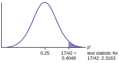
Test Statistic: \(z = 2.3163\)

Calculate the \(p\text{-value}\) using the normal distribution for proportions:

\[p\text{-value} = 0.0103\nonumber \]

In one to two complete sentences, explain what the p -value means for this problem.

If the null hypothesis is true (the proportion is 0.25), then there is a 0.0103 probability that the sample (estimated) proportion is 0.4048 \(\left(\frac{17}{42}\right)\) or more.

Use the previous information to sketch a picture of this situation. CLEARLY, label and scale the horizontal axis and shade the region(s) corresponding to the \(p\text{-value}\).

Indicate the correct decision (“reject” or “do not reject” the null hypothesis), the reason for it, and write an appropriate conclusion, using complete sentences.

Conclusion: At the 1% level of significance, the sample data do not show sufficient evidence that the percentage of fleas that are killed by the new shampoo is more than 25%.

Construct a 95% confidence interval for the true mean or proportion. Include a sketch of the graph of the situation. Label the point estimate and the lower and upper bounds of the confidence interval.

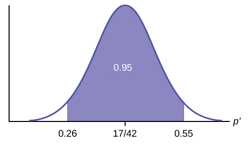
Confidence Interval: (0.26,0.55) We are 95% confident that the true population proportion p of fleas that are killed by the new shampoo is between 26% and 55%.

This test result is not very definitive since the \(p\text{-value}\) is very close to alpha. In reality, one would probably do more tests by giving the dog another bath after the fleas have had a chance to return.

Example \(\PageIndex{11}\)

In a study of 420,019 cell phone users, 172 of the subjects developed brain cancer. Test the claim that cell phone users developed brain cancer at a greater rate than that for non-cell phone users (the rate of brain cancer for non-cell phone users is 0.0340%). Since this is a critical issue, use a 0.005 significance level. Explain why the significance level should be so low in terms of a Type I error.

We will follow the four-step process.

• \(H_{0}: p \leq 0.00034\)
• \(H_{a}: p > 0.00034\)

If we commit a Type I error, we are essentially accepting a false claim. Since the claim describes cancer-causing environments, we want to minimize the chances of incorrectly identifying causes of cancer.

• We will be testing a sample proportion with \(x = 172\) and \(n = 420,019\). The sample is sufficiently large because we have \(np = 420,019(0.00034) = 142.8\), \(nq = 420,019(0.99966) = 419,876.2\), two independent outcomes, and a fixed probability of success \(p = 0.00034\). Thus we will be able to generalize our results to the population.

Figure 9.6.11.

Figure 9.6.12.

• Since the \(p\text{-value} = 0.0073\) is greater than our alpha value \(= 0.005\), we cannot reject the null. Therefore, we conclude that there is not enough evidence to support the claim of higher brain cancer rates for the cell phone users.

Example \(\PageIndex{12}\)

According to the US Census there are approximately 268,608,618 residents aged 12 and older. Statistics from the Rape, Abuse, and Incest National Network indicate that, on average, 207,754 rapes occur each year (male and female) for persons aged 12 and older. This translates into a percentage of sexual assaults of 0.078%. In Daviess County, KY, there were reported 11 rapes for a population of 37,937. Conduct an appropriate hypothesis test to determine if there is a statistically significant difference between the local sexual assault percentage and the national sexual assault percentage. Use a significance level of 0.01.

We will follow the four-step plan.

• We need to test whether the proportion of sexual assaults in Daviess County, KY is significantly different from the national average.
• \(H_{0}: p = 0.00078\)
• \(H_{a}: p \neq 0.00078\)

Figure 9.6.13.

Figure 9.6.14.

• Since the \(p\text{-value}\), \(p = 0.00063\), is less than the alpha level of 0.01, the sample data indicates that we should reject the null hypothesis. In conclusion, the sample data support the claim that the proportion of sexual assaults in Daviess County, Kentucky is different from the national average proportion.

The hypothesis test itself has an established process. This can be summarized as follows:

• Determine \(H_{0}\) and \(H_{a}\). Remember, they are contradictory.
• Determine the random variable.
• Determine the distribution for the test.
• Draw a graph, calculate the test statistic, and use the test statistic to calculate the \(p\text{-value}\). (A z -score and a t -score are examples of test statistics.)
• Compare the preconceived α with the p -value, make a decision (reject or do not reject H 0 ), and write a clear conclusion using English sentences.

Notice that in performing the hypothesis test, you use \(\alpha\) and not \(\beta\). \(\beta\) is needed to help determine the sample size of the data that is used in calculating the \(p\text{-value}\). Remember that the quantity \(1 – \beta\) is called the Power of the Test . A high power is desirable. If the power is too low, statisticians typically increase the sample size while keeping α the same.If the power is low, the null hypothesis might not be rejected when it should be.

• Data from Amit Schitai. Director of Instructional Technology and Distance Learning. LBCC.
• Data from Bloomberg Businessweek . Available online at http://www.businessweek.com/news/2011- 09-15/nyc-smoking-rate-falls-to-record-low-of-14-bloomberg-says.html.
• Data from energy.gov. Available online at http://energy.gov (accessed June 27. 2013).
• Data from Gallup®. Available online at www.gallup.com (accessed June 27, 2013).
• Data from Growing by Degrees by Allen and Seaman.
• Data from La Leche League International. Available online at www.lalecheleague.org/Law/BAFeb01.html.
• Data from the American Automobile Association. Available online at www.aaa.com (accessed June 27, 2013).
• Data from the American Library Association. Available online at www.ala.org (accessed June 27, 2013).
• Data from the Bureau of Labor Statistics. Available online at http://www.bls.gov/oes/current/oes291111.htm .
• Data from the Centers for Disease Control and Prevention. Available online at www.cdc.gov (accessed June 27, 2013)
• Data from the U.S. Census Bureau, available online at quickfacts.census.gov/qfd/states/00000.html (accessed June 27, 2013).
• Data from the United States Census Bureau. Available online at www.census.gov/hhes/socdemo/language/.
• Data from Toastmasters International. Available online at http://toastmasters.org/artisan/deta...eID=429&Page=1 .
• Data from Weather Underground. Available online at www.wunderground.com (accessed June 27, 2013).
• Federal Bureau of Investigations. “Uniform Crime Reports and Index of Crime in Daviess in the State of Kentucky enforced by Daviess County from 1985 to 2005.” Available online at http://www.disastercenter.com/kentucky/crime/3868.htm (accessed June 27, 2013).
• “Foothill-De Anza Community College District.” De Anza College, Winter 2006. Available online at research.fhda.edu/factbook/DA...t_da_2006w.pdf.
• Johansen, C., J. Boice, Jr., J. McLaughlin, J. Olsen. “Cellular Telephones and Cancer—a Nationwide Cohort Study in Denmark.” Institute of Cancer Epidemiology and the Danish Cancer Society, 93(3):203-7. Available online at http://www.ncbi.nlm.nih.gov/pubmed/11158188 (accessed June 27, 2013).
• Rape, Abuse & Incest National Network. “How often does sexual assault occur?” RAINN, 2009. Available online at www.rainn.org/get-information...sexual-assault (accessed June 27, 2013).

Contributors and Attributions

Barbara Illowsky and Susan Dean (De Anza College) with many other contributing authors. Content produced by OpenStax College is licensed under a Creative Commons Attribution License 4.0 license. Download for free at http://cnx.org/contents/[email protected] .

Statistics Made Easy

Two-Tailed Hypothesis Tests: 3 Example Problems

In statistics, we use hypothesis tests to determine whether some claim about a population parameter is true or not.

Whenever we perform a hypothesis test, we always write a null hypothesis and an alternative hypothesis, which take the following forms:

H 0 (Null Hypothesis): Population parameter = ≤, ≥ some value

H A (Alternative Hypothesis): Population parameter <, >, ≠ some value

There are two types of hypothesis tests:

• One-tailed test : Alternative hypothesis contains either < or > sign
• Two-tailed test : Alternative hypothesis contains the ≠ sign

In a two-tailed test , the alternative hypothesis always contains the not equal ( ≠ ) sign.

This indicates that we’re testing whether or not some effect exists, regardless of whether it’s a positive or negative effect.

Check out the following example problems to gain a better understanding of two-tailed tests.

Example 1: Factory Widgets

Suppose it’s assumed that the average weight of a certain widget produced at a factory is 20 grams. However, one engineer believes that a new method produces widgets that weigh less than 20 grams.

To test this, he can perform a one-tailed hypothesis test with the following null and alternative hypotheses:

• H 0 (Null Hypothesis): μ = 20 grams
• H A (Alternative Hypothesis): μ ≠ 20 grams

This is an example of a two-tailed hypothesis test because the alternative hypothesis contains the not equal “≠” sign. The engineer believes that the new method will influence widget weight, but doesn’t specify whether it will cause average weight to increase or decrease.

To test this, he uses the new method to produce 20 widgets and obtains the following information:

• n = 20 widgets
• x = 19.8 grams
• s = 3.1 grams

Plugging these values into the One Sample t-test Calculator , we obtain the following results:

• t-test statistic: -0.288525
• two-tailed p-value: 0.776

Since the p-value is not less than .05, the engineer fails to reject the null hypothesis.

He does not have sufficient evidence to say that the true mean weight of widgets produced by the new method is different than 20 grams.

Example 2: Plant Growth

Suppose a standard fertilizer has been shown to cause a species of plants to grow by an average of 10 inches. However, one botanist believes a new fertilizer causes this species of plants to grow by an average amount different than 10 inches.

To test this, she can perform a one-tailed hypothesis test with the following null and alternative hypotheses:

• H 0 (Null Hypothesis): μ = 10 inches
• H A (Alternative Hypothesis): μ ≠ 10 inches

This is an example of a two-tailed hypothesis test because the alternative hypothesis contains the not equal “≠” sign. The botanist believes that the new fertilizer will influence plant growth, but doesn’t specify whether it will cause average growth to increase or decrease.

To test this claim, she applies the new fertilizer to a simple random sample of 15 plants and obtains the following information:

• n = 15 plants
• x = 11.4 inches
• s = 2.5 inches
• t-test statistic: 2.1689
• two-tailed p-value: 0.0478

Since the p-value is less than .05, the botanist rejects the null hypothesis.

She has sufficient evidence to conclude that the new fertilizer causes an average growth that is different than 10 inches.

Example 3: Studying Method

A professor believes that a certain studying technique will influence the mean score that her students receive on a certain exam, but she’s unsure if it will increase or decrease the mean score, which is currently 82.

To test this, she lets each student use the studying technique for one month leading up to the exam and then administers the same exam to each of the students.

She then performs a hypothesis test using the following hypotheses:

• H 0 : μ = 82
• H A : μ ≠ 82

This is an example of a two-tailed hypothesis test because the alternative hypothesis contains the not equal “≠” sign. The professor believes that the studying technique will influence the mean exam score, but doesn’t specify whether it will cause the mean score to increase or decrease.

To test this claim, the professor has 25 students use the new studying method and then take the exam. He collects the following data on the exam scores for this sample of students:

• t-test statistic: 3.6586
• two-tailed p-value: 0.0012

Since the p-value is less than .05, the professor rejects the null hypothesis.

She has sufficient evidence to conclude that the new studying method produces exam scores with an average score that is different than 82.

Additional Resources

The following tutorials provide additional information about hypothesis testing:

Introduction to Hypothesis Testing What is a Directional Hypothesis? When Do You Reject the Null Hypothesis?

Featured Posts

Hey there. My name is Zach Bobbitt. I have a Masters of Science degree in Applied Statistics and I’ve worked on machine learning algorithms for professional businesses in both healthcare and retail. I’m passionate about statistics, machine learning, and data visualization and I created Statology to be a resource for both students and teachers alike.  My goal with this site is to help you learn statistics through using simple terms, plenty of real-world examples, and helpful illustrations.

One Reply to “Two-Tailed Hypothesis Tests: 3 Example Problems”

i owe u my first born child

Leave a Reply Cancel reply

Your email address will not be published. Required fields are marked *

Join the Statology Community

Sign up to receive Statology's exclusive study resource: 100 practice problems with step-by-step solutions. Plus, get our latest insights, tutorials, and data analysis tips straight to your inbox!

By subscribing you accept Statology's Privacy Policy.

If you're seeing this message, it means we're having trouble loading external resources on our website.

If you're behind a web filter, please make sure that the domains *.kastatic.org and *.kasandbox.org are unblocked.

To log in and use all the features of Khan Academy, please enable JavaScript in your browser.

AP®︎/College Statistics

Course: ap®︎/college statistics   >   unit 10.

• Idea behind hypothesis testing
• Examples of null and alternative hypotheses

Writing null and alternative hypotheses

• P-values and significance tests
• Comparing P-values to different significance levels
• Estimating a P-value from a simulation
• Estimating P-values from simulations
• Using P-values to make conclusions

• (Choice A)   H 0 : p = 0.1 H a : p ≠ 0.1 ‍   A H 0 : p = 0.1 H a : p ≠ 0.1 ‍  
• (Choice B)   H 0 : p ≠ 0.1 H a : p = 0.1 ‍   B H 0 : p ≠ 0.1 H a : p = 0.1 ‍  
• (Choice C)   H 0 : p = 0.1 H a : p > 0.1 ‍   C H 0 : p = 0.1 H a : p > 0.1 ‍  
• (Choice D)   H 0 : p = 0.1 H a : p < 0.1 ‍   D H 0 : p = 0.1 H a : p < 0.1 ‍  

with Answer, Solution | Statistical Inference - Hypothesis Testing: Solved Example Problems | 12th Business Maths and Statistics : Chapter 8 : Sampling Techniques and Statistical Inference

Chapter: 12th business maths and statistics : chapter 8 : sampling techniques and statistical inference, hypothesis testing: solved example problems.

Example 8.14

An auto company decided to introduce a new six cylinder car whose mean petrol consumption is claimed to be lower than that of the existing auto engine. It was found that the mean petrol consumption for the 50 cars was 10 km per litre with a standard deviation of 3.5 km per litre. Test at 5% level of significance, whether the claim of the new car petrol consumption is 9.5 km per litre on the average is acceptable.

Population mean μ = 9.5 km

Since population SD is unknown we consider σ = s

The sample is a large sample and so we apply Z-test

Null Hypothesis: There is no significant difference between the sample average and the company’s claim, i.e., H 0 : μ = 9.5

Alternative Hypothesis: There is significant difference between the sample average and the company’s claim, i.e., H 1 : μ ≠ 9.5 (two tailed test)

The level of significance α = 5% = 0.05

Applying the test statistic

Thus the calculated value 1.01 and the significant value or table value Z α /2 = 1.96

Comparing the calculated and table value ,Here Z < Z α /2 i.e., 1.01<1.96.

Inference:Since the calculated value is less than table value i.e., Z < Z α /2 at 5% level of sinificance, the null hypothesis H 0 is accepted. Hence we conclude that the company’s claim that the new car petrol consumption is 9.5 km per litre is acceptable.

Example 8.15

A manufacturer of ball pens claims that a certain pen he manufactures has a mean writing life of 400 pages with a standard deviation of 20 pages. A purchasing agent selects a sample of 100 pens and puts them for test. The mean writing life for the sample was 390 pages. Should the purchasing agent reject the manufactures claim at 1% level?

Population SD σ = 20 pages

The sample is a large sample and so we apply Z -test

Null Hypothesis: There is no significant difference between the sample mean and the population mean of writing life of pen he manufactures, i.e., H 0 : μ = 400

Alternative Hypothesis: There is significant difference between the sample mean and the population mean of writing life of pen he manufactures, i.e., H 1 : μ ≠ 400 (two tailed test)

The level of significance a = 1% = 0.01

Thus the calculated value |Z| = 5 and the significant value or table value Z α /2 = 2.58

Comparing the calculated and table values, we found Z > Z α /2 i.e., 5 > 2.58

Inference: Since the calculated value is greater than table value i.e., Z > Z α /2 at 1% level of significance, the null hypothesis is rejected and Therefore we concluded that μ ≠ 400 and the manufacturer’s claim is rejected at 1% level of significance.

Example 8.16

(i) A sample of 900 members has a mean 3.4 cm and SD 2.61 cm. Is the sample taken from a large population with mean 3.25 cm. and SD 2.62 cm?

(ii) If the population is normal and its mean is unknown, find the 95% and 98% confidence limits of true mean.

Population mean μ= 3.25 cm, Population SD σ = 2.61 cm

Null Hypothesis H 0 : μ = 3.25 cm (the sample has been drawn from the population mean

μ = 3.25 cm and SD σ = 2.61 cm)

Alternative Hypothesis H 1 : μ ≠ 3.25 cm (two tail) i.e., the sample has not been drawn from the population mean μ = 3.25 cm and SD σ = 2.61 cm.

Teststatistic:

∴ Z = 1.724

Thus the calculated and the significant value or table value Z α /2 = 1.96

Comparing the calculated and table values, Z < Z α /2 i.e., 1.724 < 1.96

Inference:Since the calculated value is less than table value i.e., Z > Z α /2 at 5% level of significance, the null hypothesis is accepted. Hence we conclude that the2 data doesn’t provide us any evidence against the null hypothesis. Therefore, the sample has been drawn from the population mean μ = 3.25 cm and SD, σ = 2.61 cm.

(ii) Confidence limits

95% confidential limits for the population mean μ are :

3.4− (1.96× 0.087)≤ μ ≤ 3.4+ (1.96× 0.087)

3.229≤ μ ≤ 3.571

98% confidential limits for the population mean are :

3.4− (2.33× 0.087)≤ μ ≤ 3.4+ (2.33× 0.087)

3.197 ≤ μ≤ 3.603

Therefore,95% confidential limits is (3.229,3.571) and 98% confidential limits is (3.197,3.603).

Example 8.17

The mean weekly sales of soap bars in departmental stores were 146.3 bars per store. After an advertising campaign the mean weekly sales in 400 stores for a typical week increased to 153.7 and showed a standard deviation of 17.2. Was the advertising campaign successful?

Sample size n = 400 stores

Sample SD s = 17.2 bars

Population mean μ = 146.3 bars

Since population SD is unknown we can consider the sample SD s = σ

Null Hypothesis. The advertising campaign is not successful i.e, H 0 : μ = 146.3 (There is no significant difference between the mean weekly sales of soap bars in department stores before and after advertising campaign)

Alternative Hypothesis H 1 : μ > 143.3 (Right tail test). The advertising campaign was successful

Level of significance a = 0.05

Test statistic

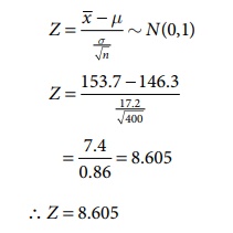
∴ Z = 8.605

Comparing the calculated value Z = 8.605 and the significant value or table value Z α  = 1.645 . we get 8.605 > 1.645

Inference: Since, the calculated value is much greater than table value i.e., Z > Z α  , it is highly significant at 5% level of significance. Hence we reject the null hypothesis H0 and conclude that the advertising campaign was definitely successful in promoting sales.

Example 8.18

The wages of the factory workers are assumed to be normally distributed with mean and variance 25. A random sample of 50 workers gives the total wages equal to ₹ 2,550. Test the hypothesis μ = 52, against the alternative hypothesis μ = 49 at 1% level of significance.

Sample size n = 50 workers

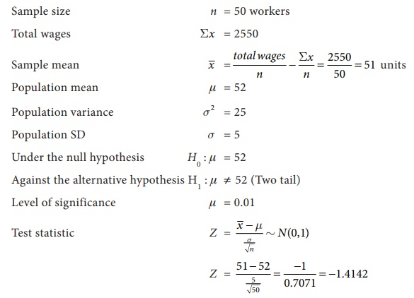
Since alternative hypothesis is of two tailed test we can take | Z | = 1.4142

Critical value at 1% level of significance is Z α /2 = 2.58

Inference: Since the calculated value is less than table value i.e., Z < Za at 1% level of significance, the null hypothesis H 0 is accepted. Therefore, we conclude 2that there is no significant difference between the sample mean and population mean μ= 52 and SD σ = 5.

Example 8.19

An ambulance service claims that it takes on the average 8.9 minutes to reach its destination in emergency calls. To check on this claim, the agency which licenses ambulance services has them timed on 50 emergency calls, getting a mean of 9.3 minutes with a standard deviation of 1.6 minutes. What can they conclude at the level of significance.

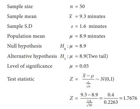
Calculated value Z = 1.7676

Critical value at 5% level of significance is Z α /2 = 1.96

Inference: Since the calculated value is less than table value i.e., Z < Z α /2 at 5% level of significance, the null hypothesis is accepted. Therefore we conclude that an ambulance service claims on the average 8.9 minutes to reach its destination in emergency calls.

Related Topics

Privacy Policy , Terms and Conditions , DMCA Policy and Compliant

Copyright © 2018-2024 BrainKart.com; All Rights Reserved. Developed by Therithal info, Chennai.