representation of water cycle

ENCYCLOPEDIC ENTRY

Water cycle.

The water cycle is the endless process that connects all of the water on Earth.

Conservation, Earth Science, Meteorology

Deer Streams National Park Mist

A misty cloud rises over Deer Streams National Park. The water cycle contains more steps than just rain and evaporation, fog and mist are other ways for water to be returned to the ground.

Photograph by Redline96

Water is one of the key ingredients to life on Earth. About 75 percent of our planet is covered by water or ice. The water cycle is the endless process that connects all of that water. It joins Earth’s oceans, land, and atmosphere.

Earth’s water cycle began about 3.8 billion years ago when rain fell on a cooling Earth, forming the oceans. The rain came from water vapor that escaped the magma in Earth’s molten core into the atmosphere. Energy from the sun helped power the water cycle and Earth’s gravity kept water in the atmosphere from leaving the planet.

The oceans hold about 97 percent of the water on Earth. About 1.7 percent of Earth’s water is stored in polar ice caps and glaciers. Rivers, lakes, and soil hold approximately 1.7 percent. A tiny fraction—just 0.001 percent—exists in Earth’s atmosphere as water vapor.

When molecules of water vapor return to liquid or solid form, they create cloud droplets that can fall back to Earth as rain or snow—a process called condensation . Most precipitation lands in the oceans. Precipitation that falls onto land flows into rivers, streams, and lakes. Some of it seeps into the soil where it is held underground as groundwater.

When warmed by the sun, water on the surface of oceans and freshwater bodies evaporates, forming a vapor. Water vapor rises into the atmosphere, where it condenses, forming clouds. It then falls back to the ground as precipitation. Moisture can also enter the atmosphere directly from ice or snow. In a process called sublimation , solid water, such as ice or snow, can transform directly into water vapor without first becoming a liquid.

Media Credits

The audio, illustrations, photos, and videos are credited beneath the media asset, except for promotional images, which generally link to another page that contains the media credit. The Rights Holder for media is the person or group credited.

Production Managers

Program specialists, specialist, content production, last updated.

April 29, 2024

User Permissions

For information on user permissions, please read our Terms of Service. If you have questions about how to cite anything on our website in your project or classroom presentation, please contact your teacher. They will best know the preferred format. When you reach out to them, you will need the page title, URL, and the date you accessed the resource.

If a media asset is downloadable, a download button appears in the corner of the media viewer. If no button appears, you cannot download or save the media.

Text on this page is printable and can be used according to our Terms of Service .

Interactives

Any interactives on this page can only be played while you are visiting our website. You cannot download interactives.

Related Resources

• Biology Article

Diagram Of Water Cycle

Table of Contents

What is the Water Cycle?

Stages of water cycle.

Water is a precious natural resource of our planet earth. It cannot be created or destroyed. The water on the earth today is the same water that existed thousands of years ago and will continue to exist years in the future.

The water cycle is an important Biogeochemical Cycle involved in the flow or circulation of water through different levels of the ecosystem. The water cycle is defined as a natural process of constantly recycling the water in the atmosphere. It is also known as the hydrological cycle or the hydrologic cycle.

During the process of the water cycle between the earth and the atmosphere, water changes into three states of matter – solid, liquid and gas.

The diagram of the water cycle is useful for both Class 9 and 10. It is one of the few important topics which are repetitively asked in the board examinations. Below is a well labelled and easy diagram of water cycle for your better understanding.

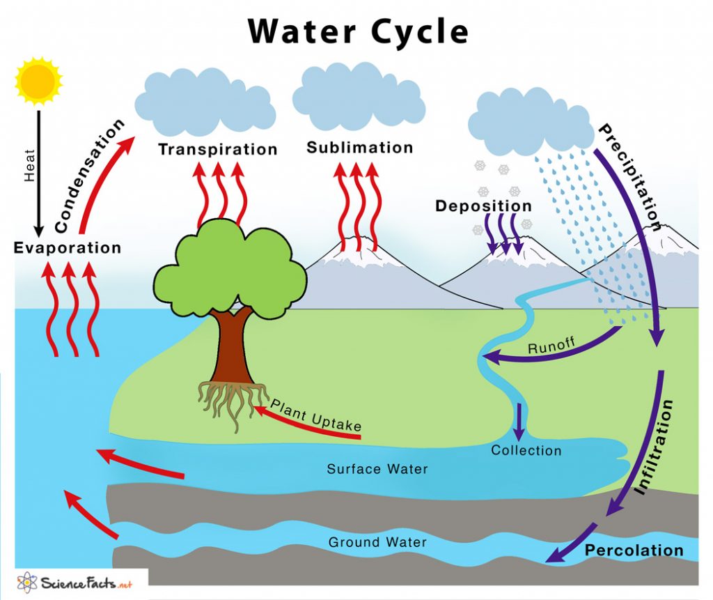
The complete water cycle is carried into four stages which are as follows: Evaporation, Condensation, Precipitation and Collection.

Evaporation

This is the initial stage of the water cycle.

The process by which water from its liquid state changes to vapour, a gaseous state, is termed as evaporation. During the water cycle, water in the water bodies get heated up and evaporates in the form of vapour, mixes with the air and disappears.

Condensation

When the evaporated water vapour loses its thermal energy, it becomes liquid through the process of condensation. Formation of clouds are examples of condensation.

Precipitation

Rain, snow, sleet, or hail are all examples of Precipitation. After the condensation, atmospheric water vapour forms sufficiently large water droplets and falls back to the earth with the help of gravity.

Deposition or Collection

This is the final stage of the water cycle. Deposition occurs when evaporated water vapour falls back to earth as precipitation. This water may fall back into the different water bodies, including oceans, rivers, ponds, lakes and even end up on the land, which in turn becomes a part of the groundwater.

Overall, the water cycle process describes how water is balanced in the atmosphere. It also plays an important role in ensuring the availability of water for all living organisms and also it has a great impact on our environment .

For more information about Water Cycle, its steps, facts and other related topics, visit us at BYJU’S Biology.

Leave a Comment Cancel reply

Your Mobile number and Email id will not be published. Required fields are marked *

Request OTP on Voice Call

Post My Comment

Thanks for your help

Thanks for your help Byjus always helps my children to understand thank u very much

Thank you! This helped so much!

Thanks a lot! This helped in my project!

It’s very helpful

• Share Share

Register with BYJU'S & Download Free PDFs

Register with byju's & watch live videos.

• school Campus Bookshelves
• menu_book Bookshelves
• perm_media Learning Objects
• login Login
• how_to_reg Request Instructor Account
• hub Instructor Commons
• Download Page (PDF)
• Download Full Book (PDF)
• Periodic Table
• Physics Constants
• Scientific Calculator
• Reference & Cite
• Tools expand_more
• Readability

selected template will load here

This action is not available.

20.2: The Water (Hydrologic) Cycle

• Last updated
• Save as PDF
• Page ID 69923
• Water cycling affects the climate, transports minerals, purifies water, and replenishes the land with fresh water.
• Water with a longer residence time, such as water in oceans and glaciers, is not available for short-term cycling, which occurs via evaporation.
• Surface water evaporates (water to water vapor) or sublimates (ice to water vapor), which deposits large amounts of water vapor into the atmosphere.
• Water vapor in the atmosphere condenses into clouds and is eventually followed by precipitation, which returns water to the earth’s surface.
• Rain percolates into the ground, where it may evaporate or enter bodies of water.
• Surface runoff enters oceans directly or via streams and lakes.

The Water (Hydrologic) Cycle

Water is essential for all living processes. The human body is more than one-half water and human cells are more than 70 percent water.  Thus, most land animals need a supply of fresh water to survive. However, when examining the stores of water on earth, 97.5 percent of it is non-potable salt water (Figure \(\PageIndex{1-2}\)). Of the remaining water, 99 percent is locked underground as water or as ice but this water is inconveniently located, mostly in Antarctica and Greenland. Shallow groundwater is the largest reservoir of usable fresh water. Less than one percent of fresh water is present in lakes and rivers, the most heavily used water resources.  If all of world's water was shrunk to the size of 1 gallon, then the total amount of fresh water would be about 1/3 cup, and the amount of readily usable fresh water would be 2 tablespoons.  

Figure \(\PageIndex{1}\):  Bar charts of the Distribution of Earth’s Water including total global water, fresh water, and surface water and other fresh water and pie charts of water usable by humans and sources of usable water reveal that only 2.5 percent of water on Earth is fresh water, and less than 1 percent of fresh water is easily accessible to living things.  Source: United States Geographical Survey Igor Skiklomanov's chapter "World fresh water resources" in Peter H. Gleick (editor), 1993, Water in Crisis: A Guide to the World's Fresh Water Resources

Many living things, such as plants, animals, and fungi, are dependent on the small amount of fresh surface water supply, a lack of which can have massive effects on ecosystem dynamics. Humans, of course, have developed technologies to increase water availability, such as digging wells to harvest groundwater, storing rainwater, and using desalination to obtain drinkable water from the ocean. Although this pursuit of drinkable water has been ongoing throughout human history, the supply of fresh water is still a major issue in modern times.

Water is the only common substance that occurs naturally on Earth in three forms: solid, liquid and gas. The hydrosphere is the area of Earth where water movement and water storage occurs.  Water reservoirs are the locations where water is stored. (Note that this term can also refer to artificial lakes created by dams.) Water is found as a liquid on the surface (rivers, lakes, oceans) and beneath the surface (groundwater), as ice (polar ice caps and glaciers), and as water vapor in the atmosphere. Figure \(\PageIndex{2}\)   illustrates the average time that an individual water molecule may spend in the Earth’s major water reservoirs.  Residence time  is a measure of the average time an individual water molecule stays in a particular reservoir.

Figure \(\PageIndex{2}\):  Average residence time that water remains in each reservoir. Water remains in organisms for about one week, in the atmosphere for 1.5 weeks, in rivers for two weeks, as soil moisture from two weeks to a year, in swamps for 1-10 years, in lakes for 10 years, in oceans and seas for 4,000 years, as groundwater for 2 weeks to 10,000 years, and in glaciers or as permafrost for 1,000-10,000 years. Image from OpenStax ( CC-BY ).

Water cycling is extremely important to ecosystem dynamics as it has a major influence on climate and, thus, on the environments of ecosystems. For example, when water evaporates, it takes up energy from its surroundings, cooling the environment. When it condenses, it releases energy, warming the environment. The evaporation phase of the cycle purifies water, which then replenishes the land with fresh water. The flow of liquid water and ice transports minerals across the globe. It is also involved in reshaping the geological features of the earth through processes including erosion and sedimentation. 

The various processes that occur during the cycling of water are illustrated in Figure \(\PageIndex{4}\).

Figure \(\PageIndex{4}\): Water from the land and oceans enters the atmosphere by evaporation or sublimation, where it condenses into clouds and falls as rain or snow. Precipitated water may enter freshwater bodies or infiltrate the soil. The cycle is complete when surface or groundwater reenters the ocean. (credit: modification of work by John M. Evans and Howard Perlman, USGS)

The water cycle is driven by the Sun’s energy as it warms the oceans and other surface waters. This leads to evaporation (water to water vapor) of liquid surface water and sublimation (ice to water vapor) of frozen water, thus moving large amounts of water into the atmosphere as water vapor. As the water vapor rises in the atmosphere, it cools and condenses. Condensation is the process in which water vapor changes to tiny droplets of liquid water. Over time, this water vapor condenses into clouds as liquid or frozen droplets and eventually leads to precipitation (rain or snow), which returns water to Earth’s surface. Most precipitation falls into the ocean. Some frozen precipitation becomes part of ice caps and glaciers. These masses of ice can store frozen water for hundreds of years or longer. Rain reaching Earth’s surface may evaporate again, flow over the surface, or percolate into the ground. Most easily observed is surface runoff: the flow of fresh water either from rain or melting ice. Runoff can make its way through streams and lakes to the oceans or flow directly to the oceans themselves.

In most natural terrestrial environments rain encounters vegetation before it reaches the soil surface. A significant percentage of water evaporates immediately from the surfaces of plants. What is left reaches the soil and begins to move down. Surface runoff will occur only if the soil becomes saturated with water in a heavy rainfall. Infiltration is the process through which water sinks into the ground and is determined by the soil or rock type through which water moves. Most water in the soil will be taken up by plant roots. The plant will use some of this water for its own metabolism, and some of that will find its way into animals that eat the plants, but much of it will be lost back to the atmosphere through a process known as evapotranspiration . Water enters the vascular system of the plant through the roots and evaporates, or transpires, through the stomata of the leaves. Water in the soil that is not taken up by a plant and that does not evaporate is able to percolate into the subsoil and bedrock. Here it forms groundwater.

Groundwater is a significant reservoir of fresh water. It exists in the pores between particles in sand and gravel, or in the fissures in rocks. Shallow groundwater flows slowly through these pores and fissures and eventually finds its way to a stream or lake where it becomes a part of the surface water again. Streams do not flow because they are replenished from rainwater directly; they flow because there is a constant inflow from groundwater below. Some groundwater is found very deep in the bedrock and can persist there for millennia. Most groundwater reservoirs, or aquifers , are the source of drinking or irrigation water drawn up through wells. In many cases these aquifers are being depleted faster than they are being replenished by water percolating down from above.

Rain and surface runoff are major ways in which minerals, including carbon, nitrogen, phosphorus, and sulfur, are cycled from land to water. More precipitation falls near the equator, and landmasses there are characterized by a tropical rainforest climate (Figure \(\PageIndex{5}\)). Less precipitation tends to fall near 20–30° north and south latitude, where the world’s largest deserts are located. These rainfall and climate patterns are related to global wind circulation cells. The intense sunlight at the equator heats air, causing it to rise and cool, which decreases the ability of the air mass to hold water vapor and results in frequent rainstorms. Around 30° north and south latitude, descending air conditions produce warmer air, which increases its ability to hold water vapor and results in dry conditions. Both the dry air conditions and the warm temperatures of these latitude belts favor evaporation. Global precipitation and climate patterns are also affected by the size of continents, major ocean currents, and mountains.

Figure \(\PageIndex{5}\):  The false-color map above shows the amount of rain that falls around the world. Areas of high rainfall include Central and South America, western Africa, and Southeast Asia. Since these areas receive so much rainfall, they are where most of the world's rainforests grow. Areas with very little rainfall usually turn into deserts. The desert areas include North Africa, the Middle East, western North America, and Central Asia. Source: United States Geological Survey Earth Forum, Houston Museum Natural Science.

An important part of the water cycle is how water varies in salinity, which is the abundance of dissolved ions in water. The saltwater in the oceans is highly saline, with about 35,000 mg of dissolved ions per liter of seawater. Evaporation is a distillation process that produces nearly pure water with almost no dissolved ions. As water vaporizes, it leaves the dissolved ions in the original liquid phase. Eventually, condensation forms clouds and sometimes precipitation. After rainwater falls onto land, it dissolves minerals in rock and soil, which increases its salinity. Rain and surface runoff are major ways in which minerals, including phosphorus and sulfur, are cycled from land to water.  Freshwater (such as lakes, rivers, and near-surface groundwater) has a relatively low salinity.

The steps of the water cycle are also explained in the video below.

Human Interactions with The Water Cycle

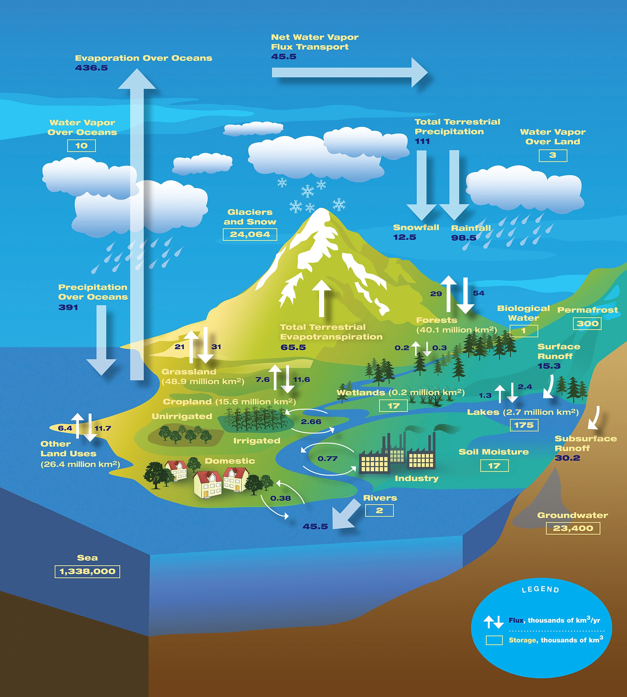
Humans alter the water cycle by extracting large amounts of freshwater from surface waters as well as groundwater. Freshwater supply is one of the most important provisioning ecosystem services on which human well-being depends. By 2000, the rate of our water extraction from rivers and aquifers had risen to almost 4000 cubic kilometers per year. The greatest use of this water is for irrigation in agriculture, but significant quantities of water are also extracted for public and municipal use, as well as industrial applications and power generation (Figure \(\PageIndex{6}\).

Figure \(\PageIndex{6}\):  The water cycle including human use of water. " The Water Cycle " by Atmospheric Infrared Sounder is available in the public domain. 

Other major human interventions in the water cycle involve changes in land cover and infrastructure development of river networks. As we have deforested areas for wood supply and agricultural development we have reduced the amount of vegetation, which naturally acts to trap precipitation as it falls and slow the rate of infiltration into the ground. As a consequence, surface runoff has increased. This, in turn, means flood peaks are greater and erosion is increased. Erosion lowers soil quality and deposits sediment in river channels, where it can block navigation and harm aquatic plants and animals. Where agricultural land is also drained these effects can be magnified. Urbanization also accelerates streamflow by preventing precipitation from filtering into the soil and shunting it into drainage systems.

Additional physical infrastructure has been added to river networks with the aim of altering the volume, timing, and direction of water flows for human benefit. This is achieved with reservoirs, weirs, aqueducts and diversion channels (Figure \(\PageIndex{7}\)). For example, so much water is removed or redirected from the Colorado River in the western United States that, despite its considerable size, in some years it is dry before reaching the sea in Mexico. In an extreme example, the Aral Sea in Central Asia has decreased to only 10% of its initial size after water was diverted for agriculture ( see this case study for more details ).

Figure \(\PageIndex{7}\):  The California Aqueduct carries water needed for agriculture from Northern California to Southern California. Image by USGS (public domain).

We also exploit waterways through their use for navigation, recreation, hydroelectricity generation and waste disposal. These activities, especially waste disposal, do not necessarily involve removal of water, but do have impacts on water quality and water flow that have negative consequences for the physical and biological properties of aquatic ecosystems.

The water cycle is key to the ecosystem service of climate regulation as well as being an essential supporting service that impacts the function of all ecosystems. Consider the widespread impacts on diverse natural and human systems when major droughts or floods occur. Consequently, human disruptions of the natural water cycle have many undesirable effects and challenge sustainable development. There are two major concerns. First, the need to balance rising human demand with the need to make our water use sustainable by reversing ecosystem damage from excess removal and pollution of water. Traditionally, considerable emphasis has been on finding and accessing more supply, but the negative environmental impacts of this approach are now appreciated, and improving the efficiency of water use is now a major goal. Second, there is a need for a safe water supply in many parts of the world, which depends on reducing water pollution and improving water treatment facilities.

Although glaciers represent the largest reservoir of fresh water, they generally are not used as a water source because they are located too far from most people (Figure \(\PageIndex{8}\)). Melting glaciers do provide a natural source of river water and groundwater. During the last Ice Age there was as much as 50% more water in glaciers than there is today, which caused sea level to be about 100 m lower. Over the past century, sea level has been rising in part due to melting glaciers. If Earth’s climate continues to warm, the melting glaciers will cause an additional rise in sea level.

Figure \(\PageIndex{8}\): Mountain Glacier in Argentina Glaciers are the largest reservoir of fresh water but they are not used much as a water resource directly by society because of their distance from most people. Source: Luca Galuzzi – www.galuzzi.it

Further "Reading"

For more information on the water cycle you might want to watch this water cycle video from USGS.

Contributors and Attributions

Modified by Kyle Whittinghill and Melissa Ha from the following sources

Samantha Fowler (Clayton State University), Rebecca Roush (Sandhills Community College), James Wise (Hampton University). Original content by OpenStax (CC BY 4.0; Access for free at https://cnx.org/contents/b3c1e1d2-83...4-e119a8aafbdd ).

• 6.6: Water Cycle by CK-12: Biology Concepts , is licensed CC BY-NC
• Biogeochemical Cycles and the Flow of Energy in the Earth System and Water Cycle and Fresh Water Supply from Sustainability: A Comprehensive Foundation by Tom Theis and Jonathan Tomkin, Editors (licensed under  CC-BY ). Download for free at  CNX .
• Water Cycle and Fresh Water Supply ,  Water Supply Problems and Solutions , and Biogeochemical Cycles from Environmental Biology  by Matthew R. Fisher (licensed under  CC-BY )
• The Water Cycle , Water Use and Distribution , and Groundwater  from  An Introduction to Geology  by Chris Johnson et al. (licensed under  CC-BY-NC-SA )
• General Microbiology  Provided by : Boundless.com.  License :  CC BY-SA: Attribution-ShareAlike  

• Why Does Water Expand When It Freezes
• Gold Foil Experiment
• Faraday Cage
• Oil Drop Experiment
• Magnetic Monopole
• Why Do Fireflies Light Up
• Types of Blood Cells With Their Structure, and Functions
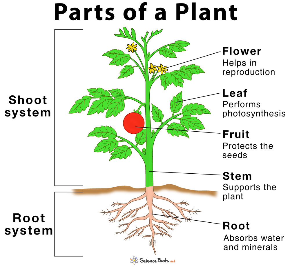
• The Main Parts of a Plant With Their Functions
• Parts of a Flower With Their Structure and Functions
• Parts of a Leaf With Their Structure and Functions
• Why Does Ice Float on Water
• Why Does Oil Float on Water
• How Do Clouds Form
• What Causes Lightning
• How are Diamonds Made
• Types of Meteorites
• Types of Volcanoes
• Types of Rocks

Water Cycle

What is the water cycle.

Water cycle, also known as the hydrologic cycle, involves a series of stages that show the continuous movement and interchange of water between its three phases – solid, liquid, and gas, in the earth’s atmosphere. The sun acts as the primary source of energy that powers   the   water cycle on earth. Bernard Palissy discovered the modern theory of the water cycle in 1580 CE.

Steps of the Water Cycle: How does it Work

1. Change from Liquid to Gaseous Phase – Evaporation and Transpiration

The heat of the sun causes water from the surface of water bodies such as oceans, streams, and lakes to evaporate into water vapor in the atmosphere. Plants also contribute to the water cycle when water gets evaporated from the aerial parts of the plant , such as leaves and stems by the process of transpiration.

2. Change from Solid to Gaseous Phase – Sublimation

Due to dry winds, low humidity, and low air pressure, snow present on the mountains change directly into water vapor, bypassing the liquid phase by a process known as sublimation.

3. Change from Gaseous to Liquid Phase – Condensation

The invisible water vapor formed through evaporation, transpiration, and sublimation rises through the atmosphere, while cool air rushes to take its place. This is the process of condensation that allows water vapor to transform back into liquid, which is then stored in the form of clouds.

Sometimes, a sudden drop in atmospheric temperature helps the water vapors to condense into tiny droplets of water that remain suspended in the air. These suspended water droplets get mixed with bits of dust in the air, resulting in fog.

4. Change from Gaseous to Liquid and Solid Phase – Precipitation and Deposition         

Wind movements cause the water-laden clouds   to collide and fall back on the earth’s surface through precipitation, simply known as rain. The water that evaporated in the first stage thus returns into different water bodies on the earth’s surface, including the ocean, rivers, ponds, and lakes. In regions with extremely cold climate with sub-zero temperatures, the water vapor changes directly into frost and snow bypassing the liquid phase, causing snowfall in high altitudes by a process known as the deposition. 

5. Return of the water back into the underground reserve – Runoff, Infiltration, Percolation, and Collection

The water that falls back on the earth’s surface moves between the layers of soil and rocks and is accumulated as the underground water reserves known as aquifers. This process is further assisted by earthquakes, which help the underground water to reach the mantle of the earth. Some amount of precipitated water flows down the sides of mountains and hills to reach the water bodies, which again evaporates into the atmosphere. During volcanic eruptions, the underground water returns to the surface of the earth, where it mixes with the surface water bodies in order to continue the cycle.

Video: Water Cycle Explained

Why is the water cycle important.

The most crucial and direct impacts of the above process on earth include:

• Making fresh water available to plants and animals, including humans, by purifying the groundwater on earth. During the water cycle, the water evaporates, leaving behind all the sediments and other dust particles. Similarly, for the sustenance of marine life, the saline range of all salt water bodies is kept within a certain permissible limit through infiltration. 
• Allowing even distribution of water on all surfaces of the earth. Water is temporarily stored as clouds in the atmosphere, whereas surface water bodies such as rivers and oceans, together with underground water, form the major permanent water reserves. 
• Causing a cooling effect on earth due to evaporation of water from surface water bodies, which help to form clouds that eventually precipitate down in the form of rain. This way water cycle affects the weather and climate of the earth.
• Ensuring some other biogeochemical cycles , including those concerning oxygen and phosphorus, to continue in nature.
• Cleaning the atmosphere by taking-away dust particles, shoot, and bacteria , thus acting as a means to purify the air we breathe.

Human Impact on Water Cycle

Human activities adversely affect the water cycle in the two following ways:

a) Deforestation : Plants play an important role in the water cycle by preventing soil erosion and thus helps to increase the groundwater level of the earth. Also, plants contribute by absorbing water from the soil, which is then released back to the atmosphere during transpiration. Deforestation adversely affects both the above processes, thus breaking the flow of the water cycle.

b) Pollution : Burning of fossil fuels acts as the major source of air pollution releasing toxic gases into the atmosphere, leading to the formation of smog and acid rain . Water from farmlands run off to the nearest water bodies carrying chemicals such as insecticides and pesticides along with them, thus causing water pollution. The presence of excessive contaminants in the atmosphere and water bodies decreases the evaporation and condensation on earth, thus adversely affecting the water cycle.

Ans. Cellular respiration is the process by which organisms take up oxygen in order to breathe and digest food. Water is utilized for breaking large molecules that release energy in the form of ATP , while in a subsequent step the water molecules are released back into the cell, which in turn returns to the atmosphere, thus affecting the water cycle.

Ans. Rivers contain more water than streams and thus contribute more to the formation of water vapor through evaporation compared to a stream.

• Water Cycle – Britannica.com
• The Water Cycle – Khanacademy.org
• Water Cycle – Noaa.gov
• What Is The Hydrologic Cycle? – Worldatlas.com
• What is the Water Cycle? – Earth.com
• The Water Cycle – Coastgis.marsci.uga.edu

Article was last reviewed on Wednesday, May 17, 2023

Related articles

One response to “Water Cycle”

The first part of the water cycle is of course evaporation and transportation, but I don’t want to focus on that, I want to focus on the 2nd step which is sublimation. Sublimation is when snow or hail, or sleet falls down on a mountain and it quickly turns into water vapor by passing the liquid phase.Now lets skip to the last phase which is RIPC

Leave a Reply Cancel reply

Your email address will not be published. Required fields are marked *

Save my name, email, and website in this browser for the next time I comment.

Popular Articles

Join our Newsletter

Fill your E-mail Address

Related Worksheets

• Privacy Policy

© 2024 ( Science Facts ). All rights reserved. Reproduction in whole or in part without permission is prohibited.

• EO Explorer

• Global Maps

The Water Cycle

Viewed from space, one of the most striking features of our home planet is the water, in both liquid and frozen forms, that covers approximately 75% of the Earth’s surface. Geologic evidence suggests that large amounts of water have likely flowed on Earth for the past 3.8 billion years—most of its existence. Believed to have initially arrived on the surface through the emissions of ancient volcanoes, water is a vital substance that sets the Earth apart from the rest of the planets in our solar system. In particular, water appears to be a necessary ingredient for the development and nourishment of life.

Earth is a water planet: three-quarters of the surface is covered by water, and water-rich clouds fill the sky. (NASA.)

Water, Water, Everywhere

Water is practically everywhere on Earth. Moreover, it is the only known substance that can naturally exist as a gas, a liquid, and solid within the relatively small range of air temperatures and pressures found at the Earth’s surface.

Water is the only common substance that can exist naturally as a gas, liquid, or solid at the relatively small range of temperatures and pressures found on the Earth’s surface. Sometimes, all three states are even present in the same time and place, such as this wintertime eruption of a geyser in Yellowstone National Park. (Photograph ©2008 haglundc. )

In all, the Earth’s water content is about 1.39 billion cubic kilometers (331 million cubic miles), with the bulk of it, about 96.5%, being in the global oceans. As for the rest, approximately 1.7% is stored in the polar icecaps, glaciers, and permanent snow, and another 1.7% is stored in groundwater, lakes, rivers, streams, and soil. Only a thousandth of 1% of the water on Earth exists as water vapor in the atmosphere.

Despite its small amount, this water vapor has a huge influence on the planet. Water vapor is a powerful greenhouse gas, and it is a major driver of the Earth’s weather and climate as it travels around the globe, transporting latent heat with it. Latent heat is heat obtained by water molecules as they transition from liquid or solid to vapor; the heat is released when the molecules condense from vapor back to liquid or solid form, creating cloud droplets and various forms of precipitation.

Water vapor—and with it energy—is carried around the globe by weather systems. This satellite image shows the distribution of water vapor over Africa and the Atlantic Ocean. White areas have high concentrations of water vapor, while dark regions are relatively dry. The brightest white areas are towering thunderclouds. The image was acquired on the morning of September 2, 2010 by SEVIRI aboard METEOSAT-9. [Watch this animation (23 MB QuickTime) of similar data to see the movement of water vapor over time.] (Image ©2010 EUMETSAT. )

For human needs, the amount of freshwater on Earth—for drinking and agriculture—is particularly important. Freshwater exists in lakes, rivers, groundwater, and frozen as snow and ice. Estimates of groundwater are particularly difficult to make, and they vary widely. (The value in the above table is near the high end of the range.)

Groundwater may constitute anywhere from approximately 22 to 30% of fresh water, with ice (including ice caps, glaciers, permanent snow, ground ice, and permafrost) accounting for most of the remaining 78 to 70%.

A Multi-Phased Journey

The water, or hydrologic, cycle describes the pilgrimage of water as water molecules make their way from the Earth’s surface to the atmosphere and back again, in some cases to below the surface. This gigantic system, powered by energy from the Sun, is a continuous exchange of moisture between the oceans, the atmosphere, and the land.

Earth’s water continuously moves through the atmosphere, into and out of the oceans, over the land surface, and underground. ( Image courtesy NOAA National Weather Service Jetstream. )

Studies have revealed that evaporation—the process by which water changes from a liquid to a gas—from oceans, seas, and other bodies of water (lakes, rivers, streams) provides nearly 90% of the moisture in our atmosphere. Most of the remaining 10% found in the atmosphere is released by plants through transpiration. Plants take in water through their roots, then release it through small pores on the underside of their leaves. In addition, a very small portion of water vapor enters the atmosphere through sublimation, the process by which water changes directly from a solid (ice or snow) to a gas. The gradual shrinking of snow banks in cases when the temperature remains below freezing results from sublimation.

Together, evaporation, transpiration, and sublimation, plus volcanic emissions, account for almost all the water vapor in the atmosphere that isn’t inserted through human activities. While evaporation from the oceans is the primary vehicle for driving the surface-to-atmosphere portion of the hydrologic cycle, transpiration is also significant. For example, a cornfield 1 acre in size can transpire as much as 4,000 gallons of water every day.

After the water enters the lower atmosphere, rising air currents carry it upward, often high into the atmosphere, where the air is cooler. In the cool air, water vapor is more likely to condense from a gas to a liquid to form cloud droplets. Cloud droplets can grow and produce precipitation (including rain, snow, sleet, freezing rain, and hail), which is the primary mechanism for transporting water from the atmosphere back to the Earth’s surface.

When precipitation falls over the land surface, it follows various routes in its subsequent paths. Some of it evaporates, returning to the atmosphere; some seeps into the ground as soil moisture or groundwater; and some runs off into rivers and streams. Almost all of the water eventually flows into the oceans or other bodies of water, where the cycle continues. At different stages of the cycle, some of the water is intercepted by humans or other life forms for drinking, washing, irrigating, and a large variety of other uses.

Groundwater is found in two broadly defined layers of the soil, the “zone of aeration,” where gaps in the soil are filled with both air and water, and, further down, the “zone of saturation,” where the gaps are completely filled with water. The boundary between these two zones is known as the water table, which rises or falls as the amount of groundwater changes.

The amount of water in the atmosphere at any moment in time is only 12,900 cubic kilometers, a minute fraction of Earth’s total water supply: if it were to completely rain out, atmospheric moisture would cover the Earth’s surface to a depth of only 2.5 centimeters. However, far more water—in fact, some 495,000 cubic kilometers of it—are cycled through the atmosphere every year. It is as if the entire amount of water in the air were removed and replenished nearly 40 times a year.

This map shows the distribution of water vapor throughout the depth of the atmosphere during August 2010. Even the wettest regions would form a layer of water only 60 millimeters deep if it were condensed at the surface. (NASA image by Robert Simmon, using AIRS & AMSU data.)

Water continually evaporates, condenses, and precipitates, and on a global basis, evaporation approximately equals precipitation. Because of this equality, the total amount of water vapor in the atmosphere remains approximately the same over time. However, over the continents, precipitation routinely exceeds evaporation, and conversely, over the oceans, evaporation exceeds precipitation.

In the case of the oceans, the continual excess of evaporation versus precipitation would eventually leave the oceans empty if they were not being replenished by additional means. Not only are they being replenished, largely through runoff from the land areas, but over the past 100 years, they have been over- replenished: sea level around the globe has risen approximately 17 centimeters over the course of the twentieth century.

Sea level has been rising over the past century, partly due to thermal expansion of the ocean as it warms, and partly due to the melting of glaciers and ice caps. (Graph ©2010 Australian Commonwealth Scientific and Research Organization. )

Sea level has risen both because of warming of the oceans, causing water to expand and increase in volume, and because more water has been entering the ocean than the amount leaving it through evaporation or other means. A primary cause for increased mass of water entering the ocean is the calving or melting of land ice (ice sheets and glaciers). Sea ice is already in the ocean, so increases or decreases in the annual amount of sea ice do not significantly affect sea level.

Blackfoot (left) and Jackson (right) glaciers, both in the mountains of Glacier National Park, were joined along their margins in 1914, but have since retreated into separate alpine cirques. The melting of glacial ice is a major contributor to sea level rise. [ Photographs by E. B. Stebinger, Glacier National Park archives (1911), and Lisa McKeon, USGS (2009).]

Throughout the hydrologic cycle, there are many paths that a water molecule might follow. Water at the bottom of Lake Superior may eventually rise into the atmosphere and fall as rain in Massachusetts. Runoff from the Massachusetts rain may drain into the Atlantic Ocean and circulate northeastward toward Iceland, destined to become part of a floe of sea ice, or, after evaporation to the atmosphere and precipitation as snow, part of a glacier.

Water molecules can take an immense variety of routes and branching trails that lead them again and again through the three phases of ice, liquid water, and water vapor. For instance, the water molecules that once fell 100 years ago as rain on your great- grandparents’ farmhouse in Iowa might now be falling as snow on your driveway in California.

The Water Cycle and Climate Change

Among the most serious Earth science and environmental policy issues confronting society are the potential changes in the Earth’s water cycle due to climate change. The science community now generally agrees that the Earth’s climate is undergoing changes in response to natural variability, including solar variability, and increasing concentrations of greenhouse gases and aerosols. Furthermore, agreement is widespread that these changes may profoundly affect atmospheric water vapor concentrations, clouds, precipitation patterns, and runoff and stream flow patterns.

Global climate change will affect the water cycle, likely creating perennial droughts in some areas and frequent floods in others. ( Photograph ©2008 Garry Schlatter. )

For example, as the lower atmosphere becomes warmer, evaporation rates will increase, resulting in an increase in the amount of moisture circulating throughout the troposphere (lower atmosphere). An observed consequence of higher water vapor concentrations is the increased frequency of intense precipitation events, mainly over land areas. Furthermore, because of warmer temperatures, more precipitation is falling as rain rather than snow.

One expected effect of climate change will be an increase in precipitation intensity: a larger proportion of rain will fall in a shorter amount of time than it has historically. Blue represents areas where climate models predict an increase in intensity by the end of the 21st century, brown represents a predicted decrease. (Map adapted from the IPCC Fourth Assessment Report.)

In parts of the Northern Hemisphere, an earlier arrival of spring-like conditions is leading to earlier peaks in snowmelt and resulting river flows. As a consequence, seasons with the highest water demand, typically summer and fall, are being impacted by a reduced availability of fresh water.

Changes in water runoff into rivers and streams are another expected consequence of climate change by the late 21st Century. This map shows predicted increases in runoff in blue, and decreases in brown and red. (Map by Robert Simmon, using data from Chris Milly, NOAA Geophysical Fluid Dynamics Laboratory.)

Warmer temperatures have led to increased drying of the land surface in some areas, with the effect of an increased incidence and severity of drought. The Palmer Drought Severity Index, which is a measure of soil moisture using precipitation measurements and rough estimates of changes in evaporation, has shown that from 1900 to 2002, the Sahel region of Africa has been experiencing harsher drought conditions. This same index also indicates an opposite trend in southern South America and the south central United States.

Shifts in the water cycle occurred over the past century due to a combination of natural variations and human forcings. From 1900 to 2002, droughts worsened in Sub-Saharan and southern Africa, eastern Brazil, and Iran (brown). Over the same period western Russia, south-eastern South America, Scandinavia, and the southern United States had less severe droughts (green). (Map adapted from the IPCC Fourth Assessment Report.)

While the brief scenarios described above represent a small portion of the observed changes in the water cycle, it should be noted that many uncertainties remain in the prediction of future climate. These uncertainties derive from the sheer complexity of the climate system, insufficient and incomplete data sets, and inconsistent results given by current climate models. However, state of the art (but still incomplete and imperfect) climate models do consistently predict that precipitation will become more variable, with increased risks of drought and floods at different times and places.

Observing the Water Cycle

Orbiting satellites are now collecting data relevant to all aspects of the hydrologic cycle, including evaporation, transpiration, condensation, precipitation, and runoff. NASA even has one satellite, Aqua, named specifically for the information it is collecting about the many components of the water cycle.

Aqua launched on May 4, 2002, with six Earth-observing instruments: the Atmospheric Infrared Sounder (AIRS), the Advanced Microwave Sounding Unit (AMSU), the Humidity Sounder for Brazil (HSB), the Advanced Microwave Scanning Radiometer for the Earth Observing System (AMSR-E), the Moderate Resolution Imaging Spectroradiometer (MODIS), and Clouds and the Earth’s Radiant Energy System (CERES).

NASA’s Aqua satellite carries a suite of instruments designed primarily to study the water cycle. (NASA image by Marit Jentoft-Nilsen.)

Since water vapor is the Earth’s primary greenhouse gas, and it contributes significantly to uncertainties in projections of future global warming, it is critical to understand how it varies in the Earth system. In the first years of the Aqua mission, AIRS, AMSU, and HSB provided space-based measurements of atmospheric temperature and water vapor that were more accurate than any obtained before; the sensors also made measurements from more altitudes than any previous sensor. The HSB is no longer operational, but the AIRS/AMSU system continues to provide high-quality atmospheric temperature and water vapor measurements.

Aqua’s AIRS and AMSU instruments measure relative humidity at multiple pressure levels, which correspond to altitude. Near the surface (100 kPa), the air above the ocean is almost saturated with water, while it is dry above Australia. It is generally drier higher in the atmosphere (60 kPa), except where convection lifts moisture aloft. At the lower edge of the stratosphere (10 kPa) the air is almost universally dry. (NASA maps by Robert Simmon, based on AIRS/AMSU data.)

More recent studies using AIRS data have demonstrated that most of the warming caused by carbon dioxide does not come directly from carbon dioxide, but rather from increased water vapor and other factors that amplify the initial warming. Other studies have shown improved estimation of the landfall of a hurricane in the Bay of Bengal by incorporating AIRS temperature measurements, and improved understanding of large-scale atmospheric patterns such as the Madden-Julian Oscillation.

In addition to their importance to our weather, clouds play a major role in regulating Earth’s climate system. MODIS, CERES, and AIRS all collect data relevant to the study of clouds. The cloud data include the height and area of clouds, the liquid water they contain, and the sizes of cloud droplets and ice particles. The size of cloud particles affects how they reflect and absorb incoming sunlight, and the reflectivity (albedo) of clouds plays a major role in Earth’s energy balance.

High, thin cirrus clouds reflect relatively little sunlight back into space compared to the amount reflected by thick cumulus clouds. This map shows the reflectivity of cirrus clouds [with a maximum of 30 percent (shown in white)] during March of 2010. (Map by Robert Simmon, using data from the MODIS Atmosphere Team. )

One of the many variables AMSR-E monitors is global precipitation. The sensor measures microwave energy, some of which passes through clouds, and so the sensor can detect the rainfall even under the clouds.

Water in the atmosphere is hardly the only focus of the Aqua mission. Among much else, AMSR-E and MODIS are being used to study sea ice. Sea ice is important to the Earth system not just as an important element in the habitat of polar bears, penguins, and some species of seals, but also because it can insulate the underlying liquid water against heat loss to the often frigid overlying polar atmosphere and because it reflects sunlight that would otherwise be available to warm the ocean.

When it comes to sea ice, AMSR-E and MODIS provide complementary information. AMSR-E doesn’t record as much detail about ice features as MODIS does, but it can distinguish ice versus open water even when it is cloudy. The AMSR-E measurements continue, with improved resolution and accuracy, a satellite record of changes in the extent of polar ice that extends back to the 1970s.

AMSR-E and MODIS also provide monitoring of snow coverage over land, another key indicator of climate change. As with sea ice, AMSR-E allows routine monitoring of the snow, irrespective of cloud cover, but with less spatial detail, while MODIS sees greater spatial detail, but only under cloud-free conditions.

As for liquid water on land, AMSR-E provides information about soil moisture, which is crucial for vegetation including agricultural crops. AMSR-E’s monitoring of soil moisture globally permits, for example, the early identification of signs of drought.

More Water Cycle Observations

Aqua is the most comprehensive of NASA’s water cycle missions, but it isn’t alone. In fact, the Terra satellite also has MODIS and CERES instruments onboard, and several other spacecraft have made or are making unique water-cycle measurements.

The Ice, Cloud, and Land Elevation Satellite (ICESat) was launched in January 2003, and it collected data on the topography of the Earth’s ice sheets, clouds, vegetation, and the thickness of sea ice off and on until October 2009. A new ICESat mission, ICESat-2, is now under development and is scheduled to launch in 2015.

ICESat’s precise observation of the surface elevation of Arctic sea ice enabled measurement of ice thickness. These images show that sea ice thinned from fall 2003 to fall 2008. Dark blue areas are thin ice, white areas are thick ice, gray regions are land, and light blue south of the ice pack represents open water. (NASA images by the NASA GSFC Scientific Visualization Studio, using ICESat data.)

The Gravity Recovery and Climate Experiment (GRACE) is a unique mission that consists of two spacecraft orbiting one behind the other; changes in the distance between the two provide information about the gravity field on the Earth below. Because gravity depends on mass, some of the changes in gravity over time signal a shift in water from one place on Earth to another. Through measurements of changing gravity fields, GRACE scientists are able to derive information about changes in the mass of ice sheets and glaciers and even changes in groundwater around the world.

These GRACE data show monthly gravity differences calculated from a 2003-2007 baseline. The big contrasts in the Amazon are due to seasonal changes in rainfall. (NASA maps by Robert Simmon, using GRACE data. )

CloudSat is advancing scientists’ understanding of cloud abundance, distribution, structure, and radiative properties (how they absorb and emit energy, including thermal infrared energy escaping from Earth’s surface). Since 2006, CloudSat has flown the first satellite-based, millimeter-wavelength cloud radar—an instrument that is 1000 times more sensitive than existing weather radars on the ground. Unlike ground-based weather radars that use centimeter wavelengths to detect raindrop-sized particles, CloudSat’s radar allows the detection of the much smaller particles of liquid water and ice in the large cloud masses that contribute significantly to our weather.

CloudSat’s radar measures the vertical distribution of clouds, such as this profile of Hurricane Julia. (NASA image by Jesse Allen, based on MODIS and CloudSat data.)

The joint NASA and French Cloud-Aerosol Lidar and Infrared Pathfinder Satellite Observations (CALIPSO) is providing new insight into the role that clouds and atmospheric aerosols (particles like dust and pollution) play in regulating Earth’s weather, climate, and air quality. CALIPSO combines an active laser instrument with passive infrared and visible imagers to probe the vertical structure and properties of thin clouds and aerosols over the globe.

CloudSat (top) and CALIPSO (lower) are two satellites providing detailed views of the structure of clouds. (NASA images by Marit Jentoft-Nilsen.)

• Ahrens, C. (1994). Meteorology: An Introduction to Weather, Climate, and the Environment. St. Paul: West Publishing Company.
• Chahine, M. (1992). The hydrological cycle and its influence on climate. Nature, 359, 373-380.
• Lutgens, F., and Tarbuck, E. (1998). The Atmosphere: An Introduction to Meteorology. Upper Saddle River: Prentice Hall.
• Kundzewicz, Z. W., Mata, L. J., Arnell, N. W., Döll, P., Kabat, P., Jiménez, B., Miller, K. A., et al. (2007). Freshwater resources and their management. In M.L. Parry, O.F. Canziani, J.P. Palutikof, P.J. van der Linden, and C.E. Hanson, (Eds.), Climate Change 2007: Impacts, Adaptation, and Vulnerability. Contribution of Working Group II to the Fourth Assessment Report of the Intergovernmental Panel on Climate Change (173–210). Cambridge: Cambridge University Press.
• Moran, J., and Morgan, M. (1997). Meteorology: The Atmosphere and the Science of Weather. Upper Saddle River: Prentice Hall.
• Parkinson, C. L. (2010). Coming Climate Crisis? Consider the Past, Beware the Big Fix. Lanham, Maryland: Rowman & Littlefield Publishers.
• Rosenzweig, C., Casassa, G., Karoly, D.J., Imeson, A., Liu, C., Menzel, A., Rawlins, A., Root, T.L., Seguin, B., and Tryjanowski, P. (2007). Assessment of observed changes and responses in natural and managed systems. In M.L. Parry, O.F. Canziani, J.P. Palutikof, P.J. van der Linden, and C.E. Hanson, (Eds.), Climate Change 2007: Impacts, Adaptation, and Vulnerability. Contribution of Working Group II to the Fourth Assessment Report of the Intergovernmental Panel on Climate Change (79-131). Cambridge: Cambridge University Press.
• Schneider, S. (1996). Encyclopedia of Climate and Weather. New York: Oxford University Press.

Atmosphere Land Life Water

Thank you for visiting nature.com. You are using a browser version with limited support for CSS. To obtain the best experience, we recommend you use a more up to date browser (or turn off compatibility mode in Internet Explorer). In the meantime, to ensure continued support, we are displaying the site without styles and JavaScript.

• View all journals
• My Account Login
• Explore content
• About the journal
• Publish with us
• Sign up for alerts
• Open access
• Published: 27 November 2023

Functional relationships reveal differences in the water cycle representation of global water models

• Sebastian Gnann   ORCID: orcid.org/0000-0002-9797-5204 1 , 2   na1 ,
• Robert Reinecke   ORCID: orcid.org/0000-0001-5699-8584 1 , 3   na1 ,
• Lina Stein   ORCID: orcid.org/0000-0002-9539-9549 1 ,
• Yoshihide Wada 4 , 5 ,
• Wim Thiery 6 ,
• Hannes Müller Schmied   ORCID: orcid.org/0000-0001-5330-9923 7 , 8 ,
• Yusuke Satoh   ORCID: orcid.org/0000-0001-6419-7330 9 ,
• Yadu Pokhrel   ORCID: orcid.org/0000-0002-1367-216X 10 ,
• Sebastian Ostberg   ORCID: orcid.org/0000-0002-2368-7015 11 ,
• Aristeidis Koutroulis   ORCID: orcid.org/0000-0002-2999-7575 12 ,
• Naota Hanasaki   ORCID: orcid.org/0000-0002-5092-7563 13 ,
• Manolis Grillakis   ORCID: orcid.org/0000-0002-4228-1803 12 ,
• Simon N. Gosling   ORCID: orcid.org/0000-0001-5973-6862 14 ,
• Peter Burek   ORCID: orcid.org/0000-0001-6390-8487 5 ,
• Marc F. P. Bierkens   ORCID: orcid.org/0000-0002-7411-6562 15 , 16 &
• Thorsten Wagener   ORCID: orcid.org/0000-0003-3881-5849 1  

Nature Water volume  1 ,  pages 1079–1090 ( 2023 ) Cite this article

6387 Accesses

3 Citations

94 Altmetric

Metrics details

• Environmental impact
• Water resources

Global water models are increasingly used to understand past, present and future water cycles, but disagreements between simulated variables make model-based inferences uncertain. Although there is empirical evidence of different large-scale relationships in hydrology, these relationships are rarely considered in model evaluation. Here we evaluate global water models using functional relationships that capture the spatial co-variability of forcing variables (precipitation, net radiation) and key response variables (actual evapotranspiration, groundwater recharge, total runoff). Results show strong disagreement in both shape and strength of model-based functional relationships, especially for groundwater recharge. Empirical and theory-derived functional relationships show varying agreements with models, indicating that our process understanding is particularly uncertain for energy balance processes, groundwater recharge processes and in dry and/or cold regions. Functional relationships offer great potential for model evaluation and an opportunity for fundamental advances in global hydrology and Earth system research in general.

Similar content being viewed by others

Climate change will affect global water availability through compounding changes in seasonal precipitation and evaporation

Reconciling historical changes in the hydrological cycle over land

Multi-model Hydroclimate Projections for the Alabama-Coosa-Tallapoosa River Basin in the Southeastern United States

Global water models—including hydrological, land surface and dynamic vegetation models 1 —have become increasingly relevant for policymaking and in scientific studies. The Sixth Assessment Report 2 of the Intergovernmental Panel on Climate Change draws heavily on results from global water models, which provide information about climate change impacts on hydrological variables including soil moisture 3 , streamflow 4 , terrestrial water storage 5 and groundwater recharge 6 . Some of these models are already embedded in global water information services to provide information to a wide array of stakeholders, such as the Global Groundwater Information System 7 or the African Flood and Drought Monitor 8 . Because measurements of many hydrological variables are very sparse and insufficient for large-scale analyses, global water models are regularly used in scientific studies to provide globally coherent estimates of variables such as groundwater recharge and groundwater storage change 9 , 10 . Global water models are also an integral part of Earth system models, and a realistic representation of the water cycle is essential for simulating the role of water within and across the different components of the Earth system 11 .

The Intergovernmental Panel on Climate Change’s Sixth Assessment Report 2 concludes from an analysis of currently available global water model projections that ‘uncertainty in future water availability contributes to the policy challenges for adaptation, for example, for managing risks of water scarcity’. Whereas some of this uncertainty stems from projected and observed climatic forcing, considerable uncertainty stems from global water models themselves 4 , 6 , 12 , 13 , 14 . For instance, Beck et al. 13 found distinct inter-model performance differences when comparing simulated and observed streamflow for ten global water models driven by the same forcing. To illustrate this uncertainty, we show how 30-year (climatological) averages of actual evapotranspiration, groundwater recharge and total runoff vary globally on the basis of outputs from eight models driven by the same forcing (Fig. 1a–c ; Methods). We find substantial disagreement among models, as indicated by high coefficients of variation, particularly for groundwater recharge and total runoff. We further show which model deviates most from the ensemble mean and find that there is not one model that consistently deviates the most (Fig. 1d–f ). Whereas this analysis cannot tell us which models perform better or worse, it suggests that it is not straightforward to single out a model for a certain flux or a certain region, which warrants a more in-depth evaluation.

a – c , Left: maps showing the coefficient of variation, calculated per grid cell as the ensemble standard deviation divided by the ensemble mean of eight global water models for different water fluxes: actual evapotranspiration ( a ), groundwater recharge ( b ) and total runoff ( c ). Lighter areas (‘blank spaces’) indicate high coefficients of variation (CoV) values and thus show where models disagree most. d – f , Right: maps showing which model deviates most from the ensemble mean for each grid cell for different water fluxes: actual evapotranspiration ( d ), groundwater recharge ( e ) and total runoff ( f ). Dark grey areas in d – f indicate that multiple models deviate similarly strongly from the ensemble mean. Empty, blank areas in d – f indicate that no model deviates strongly from the ensemble mean. The percentages shown in d – f refer to the fraction of grid cells (not land area) covered by each model. Greenland is masked out for the analysis.

Most evaluation strategies compare model outputs to historical observations over the area for which the observation is representative. This can be at the plot (for example, flux towers), catchment (for example, gauging stations) or grid cell (for example, gridded remote sensing products) scale. Such approaches are necessary but not sufficient to robustly evaluate global models 15 . First, these approaches compare simulated and observed values location by location and are therefore limited to potentially improving a model for that location; however, given that large fractions of the global land area are ungauged, we require methods that can extract and transfer information from gauged to ungauged locations 16 . Second, relevant information for model evaluation might not just lie in comparing the magnitudes of simulated and observed values in a single location but rather in how a variable varies along a spatial gradient 17 . And third, comparison with historical observations does not guarantee that a model reliably predicts system behaviour under changing conditions 18 . Rather than evaluating global models in essentially the same way as catchment-scale models, evidence of different large-scale hydrological relationships presents us with an opportunity for a different evaluation strategy that is inherently large-scale but so far rarely exploited.

Towards evaluation using functional relationships

Reviewing the hydrological literature reveals a range of relationships 19 that, if they appear in empirical data, should also appear in models (and vice versa). Such relationships often capture behaviour that is not prescribed by small-scale processes but rather emerges through the interaction of these processes (or model components) at large scales. The perhaps most prominent example is the Budyko framework 20 , which describes the long-term partitioning of precipitation into evapotranspiration and streamflow solely as a function of the aridity index. Another example are so-called elasticities of streamflow to changing climatic drivers (for example, precipitation or temperature), which provide an observation-based constraint on climate change effects on streamflow 21 , 22 . A third example are empirical relationships between annual rainfall and runoff, which can be affected differently by prolonged drought; in Australia, some catchments have shown similar rainfall–runoff relationships before and after the Millennium Drought, while other catchments have transitioned to a new stable state 23 . The search for robust relationships that characterize the functioning of hydrological systems is in itself a great scientific challenge 19 , but such functional relationships also provide an excellent yet poorly explored opportunity for the evaluation of global water models.

We define the term function as the actions of (hydrological) systems on the inputs that enter them, such as partition, storage and release of water and energy 24 , 25 . Accordingly, we define functional relationships as relationships between two or more variables that characterize these functions. Such relationships often focus on forcing, state and response variables that are expected to be causally related (for example, precipitation and runoff), and they can focus on both temporal variability at a single location and (as used here) spatial variability across multiple locations. Functional relationships need not be uniquely defined and are typically characterized by substantial scatter due to other (secondary) controlling variables, local variability or uncertainty.

Whereas functional relationships have been used before to evaluate land surface, forest and Earth system models—for example, by analysing relationships between soil moisture and evaporation and runoff 26 , 27 , 28 , 29 or between precipitation and other atmospheric drivers and vegetation productivity 30 , 31 , 32 —their potential for evaluating global water models has not yet been sufficiently explored. The use of functional relationships is currently scattered among the hydrological literature (for example, refs. 33 , 34 , 35 ) and has not been formalized into an evaluation framework. There is a pressing need to develop a ‘theory of evaluation’ 36 that does justice to the nature of global models, the purposes for which they are used and their growing relevance for society 37 . Functional relationships have the potential to be a central building block of such a theory of evaluation, and below we show how they can help shed new light on model behaviour.

Here we focus on functional relationships that capture the spatial co-variability of forcing and response variables. Rather than focusing on a process-by-process comparison that can quickly become unmanageable 28 , functional relationships can capture emergent patterns and shift the focus to identifying the dominant controls on the variables of interest. Especially the relationships between water and energy availability and the major water fluxes leaving the land surface—evaporation and runoff—have been frequently studied 20 , 38 , providing an excellent starting point for model evaluation. In addition, functional relationships that focus on spatial patterns offer several advantages. First, such relationships are well suited for the analysis of global models due to their spatially distributed nature, which means that these relationships can be readily obtained from comparing values from multiple grid cells. Second, spatial relationships can be calculated based on long-term averages, which for some variables are often the only observations available (for example, for groundwater recharge 39 , 40 ). And third, such relationships can capture how hydrological variables co-vary across large scales and thus offer the potential for model improvement over large areas, including locations that lack observations.

In this analysis, we investigate how long-term averages of two forcing and three response variables co-vary spatially, leading to six variable pairs overall. The forcing variables are precipitation P and net radiation N (the available water and energy, respectively), and the response variables are actual evapotranspiration E a , groundwater recharge R and total runoff Q (three key water fluxes). We analyse forcing–response relationships based on 30-year (climatological) averages (1975–2004; all in mm per year) from eight global water models (CLM4.5, CWatM, H08, JULES-W1, LPJmL, MATSIRO, PCR-GLOBWB and WaterGAP2) from phase 2b of the Inter-Sectoral Impact Model Intercomparison Project (ISIMIP 2b 41 ). In addition, we use observational datasets, observation-driven machine learning products and the semi-empirical equation introduced by Budyko 20 to calculate functional relationships between the same variables as for the models as benchmarks (Table 1 ). To explore regional variability in functional relationships 38 , we divide the world into four climatic regions: wet–warm (18% of modelled area), wet–cold (15%), dry–cold (24%) and dry–warm (43%), shown in Fig. 2d . Details can be found in the Methods section.

a , Scatter plots between precipitation and groundwater recharge for PCR-GLOBWB and WaterGAP2. Owing to space constraints, we focus on a few examples with differing relationships. Scatter plots for all variable pairs are shown in Supplementary Figs. 15 – 20 . Each dot represents one grid cell and is based on the 30-year average of each flux. Spearman rank correlations ρ s measure the strength of the relationship between forcing and response variables and are calculated for all grid cells within a climate region. The lines connect binned medians (ten bins along the x axis with equal amount of points per bin) for each region. b , The climate regions are shown. The grey dashed line shows the 1:1 line, indicating the water limit assuming all water is supplied by precipitation.

Disagreement in functional relationships between models

We can visually assess relationships between forcing ( P ,  N ) and response variables ( E a ,  R ,  Q ) by inspecting scatter plots where each point represents one grid cell (or observation); this is shown for precipitation and groundwater recharge in Fig. 2a . We first take a closer look at the shapes of the functional relationships, indicated by the coloured lines in Fig. 2a . Later we will also quantify the strength of the relationships using Spearman rank correlations ρ s . We limit ourselves to a qualitative discussion, given that fitting an equation would mean that we would have to assume a functional form. We report mean values and slopes (obtained via linear regression) for each region in Supplementary Tables 4 – 7 , which quantitatively support our visual assessment. Figure 3 shows connected binned median values for precipitation and the three water fluxes for all models and observational datasets (Table 1 ), separated by climate region. A similar plot for net radiation and the three water fluxes is shown in Extended Data Fig. 1 .

Average functional relationships based on models and benchmark datasets among precipitation P and actual evapotranspiration E a , groundwater recharge R and total runoff Q , respectively. The coloured lines represent one model each, the grey-black lines represent different observational datasets, labelled on the outer-right panels. The MacDonald groundwater recharge dataset contains only enough data values for the dry–warm region and is thus only shown there. The lines connect binned medians (ten bins along the x axis with equal amount of points per bin) for each climate region. The grey dashed line shows the 1:1 line, indicating the water limit assuming all water is supplied by precipitation. Note that the graphs do not show the full range for some curves to better illustrate the model differences.

While the P – E a relationships look similar in shape, they can differ greatly in magnitude (Fig. 3 ). They increase rather linearly in dry (water-limited) regions and increase initially in wet (energy-limited) regions and then level off as they reach an energy limit that bounds actual evapotranspiration. The limit differs greatly between models, varying up to about 400 mm per year in wet–warm regions. Because all models are forced with the same total radiation, this difference is related to the way the models translate total radiation into net radiation and how they then use net radiation to calculate actual evapotranspiration. There is no obvious connection between this difference and the different potential evapotranspiration schemes used 42 , potentially because the models, while forced with the same climate inputs, differ in the way they parameterize the land surface (for example, land use, soils). In dry regions, actual evapotranspiration is mostly limited by precipitation, a forcing dataset that is the same for all models, resulting in less variability. The Budyko equation and the FLUXCOM 43 dataset suggest, in line with literature estimates 44 , that most models underestimate actual evapotranspiration, often greatly so (Supplementary Tables 4 and 5 ). However, we note that FLUXCOM probably overestimates actual evapotranspiration, especially in dry–warm regions, because it considers only vegetated areas 43 . Overall, the disagreement in modelled actual evapotranspiration, particularly visible in energy-limited regions, suggests substantial differences in the way models estimate the energy available for evapotranspiration.

Most P – R relationships increase monotonically, but the shape, the slope and the threshold at which some models start to produce groundwater recharge are very different (Fig. 3 ). For instance, in dry–warm regions, some models produce essentially no groundwater recharge even if precipitation is above 1,000 mm per year, while others produce over 200 mm per year. In dry–warm regions, we have by far the most extensive database on groundwater recharge 39 , 40 , and the observations fall (apart from those at very high precipitation values) within the range of the models. In wet–warm regions, we find the largest disagreement between models and observations, which suggest lower (higher) groundwater recharge rates for higher (lower) precipitation. Whereas this shows the benefit of using an ensemble rather than a single model, even a large ensemble spread does not always capture the observed relationships. The large spread further suggests that many models greatly over- or underestimate groundwater recharge rates and consequently greatly over- or underestimate how much groundwater contributes to evapotranspiration and streamflow 45 . These differences in slope, visible for all climate regions, reflect very different spatial sensitivities to changes in precipitation. Whether temporal sensitivities are similar can only be hypothesized given that no global observational dataset with groundwater recharge time series is available but would imply very different responses to projected changes in precipitation.

The P – Q relationships look similar in shape and mostly increase monotonically, especially for wet regions (Fig. 3 ). The relative differences are larger for dry places, commonly perceived as regions where runoff is more difficult to model 46 . The model and benchmark relationships disagree particularly strongly in dry–cold regions. There, the GSIM 47 , 48 dataset shows a variable relationship between total runoff and precipitation, whereas the GRUN 49 dataset shows almost no increase with increasing precipitation. Overall, GSIM, GRUN and the Budyko equation indicate, in line with an earlier evaluation 50 , that most models produce too much total runoff. This parallels recent findings that Earth system models predict higher runoff increases due to climate change than observations suggest 22 . The overestimation in total runoff is complementary to the underestimation of actual evapotranspiration and shows that most models partition too much precipitation into runoff rather than evapotranspiration.

Diverging dominance of forcing on response variables

To quantitatively compare the strength of the forcing–response relationships, we use Spearman rank correlations ρ s . A rank correlation close to 1 (or −1) indicates that the spatial variability in the forcing variable almost completely explains the spatial variability in the response variable, as can be seen in Fig. 2a for WaterGAP2. A rank correlation closer to 0 indicates that other factors control the response (for example, other input or model parameters describing the land surface), as can be seen in Fig. 2a for PCR-GLOBWB. We stress that a high correlation is not a measure of goodness of fit. Considerable scatter and correspondingly low correlations might indeed be characteristic for many relationships, and if models overestimate how strongly a forcing variable controls a model output, this also indicates unrealistic behaviour. Calculating rank correlations for all variable pairs, we find that the models differ substantially among each other and in comparison to observations (Fig. 4 ; rank correlations for all benchmark datasets and models are listed in Table 1 and Supplementary Table 3 , respectively).

a – f , Spearman rank correlations ρ s between forcing variables (precipitation ( a , c , e ), net radiation ( b , d , f )) and water fluxes (actual evapotranspiration ( a , b ), groundwater recharge ( c , d ) and total runoff ( e , f )), divided into different climate regions. Net radiation for LPJmL and PCR-GLOBWB is not available and is estimated as the median of the other models (per grid cell). The lines connecting the dots are only there as a visual aid. The numbered triangles show rank correlations based on benchmark datasets (grey background) and the Budyko equation, with numbers indicating the corresponding data source (Table 1 ). Observation-based rank correlations are shown only if they are based on more than 50 data points.

For precipitation and actual evapotranspiration (Fig. 4a ), the models show the same ranking between climate regions and rather small differences in magnitude, indicating that actual evapotranspiration is strongly constrained by the available water in all models. The model-based correlations are higher in dry regions ( ρ s  = 0.74–0.98) than in wet regions (0.57–0.83), reflecting water and energy limitations. The Budyko equation assumes complete dependence on aridity (here defined as N / P ). It thus predicts higher correlations overall and mainly distinguishes between wet (0.83–0.84) and dry (0.98–1.00) regions but, unlike models and FLUXCOM, not between cold and warm regions. The Budyko equation should thus be seen as a useful comparison but not as the ‘correct’ model, given that different studies have shown that snow 51 , climate seasonality 52 , vegetation type 53 , inter-catchment groundwater flow 54 and human impacts 55 can affect the long-term water balance beyond aridity.

We find much variability for net radiation and actual evapotranspiration (Fig. 4b ). There is no obvious correspondence between the potential evapotranspiration schemes used 42 (for example, Priestley–Taylor for LPJmL and WaterGAP2 or Penman–Monteith for JULES-W1 and CWatM) and the rank correlations, implying that other factors play a more important role (also, refs. 14 , 56 ). Both the Budyko equation and FLUXCOM show very high correlations for all wet places (0.93–0.99), indicating a strong energy limitation 57 , underestimated by many models (especially CWatM and MATSIRO). FLUXCOM shows a stronger N – E a relationship (Fig. 4b ) in dry–cold places than all models and the Budyko equation, while it shows a weaker P – E a relationship (Fig. 4a ) there. This could be due to an uncertain representation of energy balance processes in cold regions, possibly related to interactions between snow-affected albedo and evapotranspiration 58 , 59 , sublimation 60 or the aerodynamic component of potential evapotranspiration 61 .

For precipitation and groundwater recharge (Fig. 4c ), some models (CLM4.5, MATSIRO, WaterGAP2 and H08) show high to very high correlations (0.71–0.95) for all climate regions, suggesting that precipitation is the dominant control on groundwater recharge across all climate regions in these models. Other models (CWatM, JULES-W1, LPJmL, PCR-GLOBWB) show much lower and more variable correlations (0.35–0.85), suggesting different controls on groundwater recharge (for example, model structural decisions and parameterizations). H08 and WaterGAP2 use the same approach to calculate groundwater recharge 42 and they show almost identical rank correlations, indicating that the functional relationships might be relatable to the model structure in this case. Recent studies have shown a strong influence of precipitation and aridity on groundwater recharge 39 , 40 , 45 , and using the same datasets, we also find high to very high correlations in dry–warm regions (0.74–0.84). In these often highly water-limited regions, precipitation appears to be the dominant control on groundwater recharge. Besides climate, perceptual models of groundwater recharge generation usually include soil characteristics, topography, land use and geology 62 , 63 . This might explain why observations show a more scattered P – R relationship, particularly in wet–warm regions (−0.06).

For precipitation and total runoff (Fig. 4e ), WaterGAP2 and PCR-GLOBWB both show lower correlations (0.52–0.75) than the other models (0.58–0.95). WaterGAP2 is the only model here that is calibrated against streamflow observations 42 , which might explain why it shows the lowest rank correlations for total runoff. The Budyko framework assumes that long-term runoff only depends on aridity and thus shows higher correlations (0.87–0.99) than the benchmark datasets (0.27–0.94) and most models (0.52–0.95). Because factors other than aridity can influence total runoff 51 , 52 , 53 , 54 and given that GSIM tends to show lower correlations overall (0.32–0.80), models that show correlations as high as the Budyko equation probably overestimate how strongly precipitation controls total runoff. Similar to the shapes of the functional relationships (Fig. 3 ),we generally find the largest differences in both models and datasets in dry–cold regions, where GRUN and GSIM show particularly low correlations (0.27 and 0.32).

For net radiation and both groundwater recharge and total runoff (Fig. 4d,f ), we find high variability and mostly positive correlations. The models probably produce more groundwater recharge and total runoff in regions with higher net radiation because precipitation is also higher in these regions (Supplementary Fig. 1 ). Whereas it is difficult to interpret these correlations, the large variability still suggests considerable differences between models.

Focus areas for model improvement

Our analysis has revealed substantial disagreement between models and between models and observations, questioning the robustness of model-based studies and impact assessments, especially if only a single model is used. The energy balance, from total radiation to actual evapotranspiration, appears to be poorly represented, indicated by a different energy limit (Fig. 3 ), a general underestimation of actual evapotranspiration and widely varying N – E a relationships (Fig. 4 ). This warrants a closer look in future studies, as a realistic depiction of energy balance and evaporation processes is critical for climate change studies 57 , 58 . We find the largest disagreement for groundwater recharge, which is arguably the least understood process and poorly constrained by sparse observations 39 , 40 . The inter-model differences in groundwater recharge can be much larger than the differences in actual evapotranspiration and must therefore have other reasons. To better constrain the large variability between models, we need to improve our understanding of the dominant controls on groundwater recharge at large scales 64 . This knowledge is important for assessments of sustainable use of groundwater resources 9 , 10 , for groundwater modelling studies that use groundwater recharge from global water models as input 65 and for understanding the sensitivity of groundwater recharge to changing climatic drivers 6 . Most models overestimate total runoff and we find the largest disagreement for total runoff in dry–cold regions. This echoes existing literature 1 , 12 , 22 , 50 and highlights the need for model refinement in dry and/or cold regions, which are under-researched and strongly affected by climate change 46 . To explore more in-depth how snow processes affect the water balance, future studies could focus on functional relationships in snow-dominated regions by specifically delineating these regions using the fraction of precipitation falling as snow or snow cover extents.

Towards an inventory of robust functional relationships

We have used different observational datasets, observation-driven machine learning products and the Budyko equation 20 to derive empirical and theory-based functional relationships, but challenges remain. Observation-driven machine learning products 43 , 49 are not raw observations and may reflect their upscaling methods rather than the underlying natural distribution but serve as useful benchmarks in the absence of direct observations (for example, because of limited numbers of FLUXNET sites 66 ). The Budyko equation 20 is a climate-only model and thus provides a useful benchmark but neglects other influences on the long-term water balance. The observations themselves and the forcing data paired with them are also associated with uncertainty, even though most of the relationships used here appear to be relatively robust (Methods includes an extended discussion). Yet especially for variables with small numbers of observations, it is challenging to provide robust observation-based constraints for certain regions (Table 1 ). For example, groundwater recharge measurements have almost entirely been made in dry–warm regions (97% of MacDonald data 40 and 92% of Moeck data 39 ), leaving groundwater recharge in other regions poorly constrained. On the other hand, most streamflow measurements have been taken in wet regions (60% of GSIM data used here), and globally there is a placement bias of stream gauges towards wet regions 67 , even though—according to our classification—short of two-thirds of the global land area are defined as dry. Instead of taking new measurements to understand a specific place, new measurements would have much more leverage if they would help us to also understand other places, for example, by filling an observational gap along a climatic gradient (that is, in functional space). In addition, more quality-controlled datasets with uncertainty estimates 40 are critical to obtain realistic uncertainty estimates for functional relationships. This would ultimately allow us to obtain robust ranges of functional behaviour that we can benchmark our models against.

The functional relationships studied here appear to be robust with respect to modelled human impacts, probably because we investigated long-term averages over large regions where climatic controls on the selected hydrological variables dominate (Supplementary Figs. 26 – 30 ). Yet for different variables, especially when studied at shorter temporal and smaller spatial scales, human impacts might have a considerable effect on functional relationships. The effects of human impacts might be investigated by studying strongly managed and near-natural regions separately 68 . Indeed, comparing functional relationships between human impacted and natural regions would be an excellent strategy to assess the degree of human alteration of the natural water cycle. In addition, relationships that specifically focus on human impacts, such as relationships between irrigated areas and irrigation water withdrawals 69 , might be used to better understand the representation of human impacts in models.

Whereas visual comparison (focusing on the shape of the relationships) and rank correlations (focusing on the strength of the relationships) have exposed clear differences between models and observations, our approach here should be seen as a first step. There are other ways to describe the relationships analysed here, for example, by characterizing thresholds or nonlinearities (visible in Fig. 3 ). Metrics such as rank correlations also require careful interpretation. For example, positive correlations between net radiation and groundwater recharge probably arise because precipitation and net radiation are positively correlated and thus do not imply a causal relationship. The interpretation of empirical relationships should therefore be backed up by process knowledge or extended by methods that allow for discovery of causal relationships 70 . Physics-aware machine learning might be powerful in that respect, as it combines domain knowledge with versatile pattern recognition 71 . Beyond the relationships investigated here, we anticipate that exploring temporal relationships (for example, using elasticities 21 , 22 or shifts in P – Q relationships 23 ), dividing the landscape into additional categories (for example, hydrobelts 72 ) and including other variables, such as state variables or stores (for example, soil moisture, terrestrial water storage), will provide additional insights.

Conclusions

As our models grow in complexity, encompassing more processes and covering larger spatial and temporal scales, we need a concurrent development of model evaluation strategies: an evaluation framework for large-scale models. Central to such an evaluation framework should be functional relationships, which shift the focus away from matching historical records in specific locations to a more diagnostic and process-oriented evaluation of model behaviour 36 . Functional relationships allow us to focus on larger-scale assessments, to relate places to each other and to explore if dominant controls in models are consistent with observations, theory and expectations (that is, our perceptual model 73 ). This understanding is critical for ensuring that models faithfully represent real-world systems, ultimately leading to more credible projections of environmental change impacts. Eventually, expanding our range of functional relationships in hydrology, constrained by various observational datasets and expert knowledge, would give us a knowledge base of realistic system behaviour that could be used to evaluate models, diagnose model deficiencies and weight model ensembles, comparable to the use of emergent constraints in climate modelling 37 .

Both our approach and our findings have implications beyond hydrology. First, the terrestrial water cycle plays a central role in the Earth system and is often strongly coupled to other components, such as the biosphere, lithosphere and atmosphere and human activities (for example, refs. 74 , 75 , 76 ). More realistic simulations of the global water cycle therefore also enable us to better clarify how it influences and is influenced by other Earth system components. Methodologically, functional relationships are not limited to applications in hydrology. In fact, land surface, forest and Earth system models 26 , 27 , 28 , 29 , 30 , 31 , 32 have already been studied in similar fashions, though a broader application of this approach has so far been missing. As indicated by recent studies 76 , 77 , functional relationships provide an excellent opportunity to study the interactions between hydrology and, for example, terrestrial ecosystems, and thus represent a tool that can be used across disciplines.

Beyond model evaluation, functional relationships invite us to think about how the global water cycle functions, what we know, what we do not know and what that means for a future under climate change 73 . Our results suggest that improved process understanding will be particularly important for energy balance processes, groundwater recharge processes and generally in dry and/or cold regions. So how can we improve our process understanding? In 1986, Eagleson 78 stated that ‘science advances on two legs, analysis and experimentation, and at any moment one is ahead of the other. At the present time advances in hydrology appear to be data limited’. For some processes, this still seems to be the case. But clearly, we have a wealth of data available and might ask ourselves: are we extracting all of the information from the observations we have? On the basis of the data we have, what and where should we measure next? And are there functional relationships in hydrology yet to be found 19 ? Even if the search for such relationships is challenging, it will be a fruitful and exciting endeavour for global hydrology.

Model data retrieval and processing

We analysed 30-year (climatological) averages (1975–2004) from eight global water models 41 : CLM4.5 79 , CWatM 80 , H08 81 , JULES-W1 82 , LPJmL 83 , MATSIRO 84 , PCR-GLOBWB 85 and WaterGAP2 86 . The model simulations were carried out following the ISIMIP 2b protocol and here we used model outputs forced with the Earth system model HadGEM2-ES under historical conditions (historical climate and CO 2 concentrations). We note that the specific forcing chosen does not appear to influence model-based functional relationships (see below). We used precipitation P (ISIMIP variable name p r ), net radiation N (not an official ISIMIP output), actual evapotranspiration E a (ISIMIP variable name e v a p ), groundwater recharge R (ISIMIP variable name q r ) and total runoff Q (ISIMIP variable name q t o t ). Note that Q here refers to runoff generated on the land fractions (and not surface water bodies) of each grid cell and does not include upstream inflows, which allows for comparison to grid cell P . P , E a , R , and Q were downloaded from https://data.isimip.org/ . Net radiation N is not an official ISIMIP output and was provided by the individual modelling groups. It is not available for all models, so we used the ensemble median per grid cell for models without N data. We converted all fluxes to mm per year and removed E a values larger than 10,000 mm per year and set R values smaller than 0 to 0. Note that our analysis excludes Greenland and Antarctica. A more detailed description is given in the Supplementary Information .

CoV and most deviating model maps

For each grid cell, we used the 30-year averages of the eight models (that is, the model ensemble) and calculated the ensemble standard deviation divided by the ensemble mean. Maps of the standard deviation are shown in the Supplementary Information (Supplementary Figs. 8 – 10 ). To see which model dominates the ensemble spread, we checked for each grid cell which model shows the largest absolute difference (denoted by d 1 ) from the ensemble mean (denoted by μ ). To see if multiple models dominate the ensemble spread, we also checked for each grid cell which model shows the second-largest absolute difference (denoted by d 2 ) from the ensemble mean. If the relative difference between the largest and the second-largest difference is less than 20%, that is ( d 1  −  d 2 )/ d 1  < 0.2, the grid cell falls into the category ‘multiple’. If the relative difference between the most deviating model and the ensemble mean is less than 20%, that is d 1 / μ  < 0.2, the grid cell is counted as having no most deviating model (empty areas on Fig. 1d–f ).

Functional relationships

To visualize the shape of the functional relationships, we binned the data in each climate region into ten bins (along the x axis) with an equal amount of points, calculated the median per bin and connected the obtained median value. For groundwater recharge, we used only five bins because there are so few values. Note that the non-gridded observational datasets do not have the same spatial distribution as the gridded datasets and the models and thus do not have the same distribution of forcing variables. Their bins can therefore span different ranges of the forcing variables. As a metric for the strength of the functional relationships, we calculate Spearman rank correlations ρ s between model inputs and outputs per climate region, a measure of the monotonicity between two variables that is robust to outliers. We use the following categories for correlations: negative correlation (<0), no to low correlation (0 to 0.25), medium correlation (0.25–0.5), high correlation (0.5–0.75), very high correlation (0.75–1.0). We also show mean fluxes and slopes obtained through linear regression in Supplementary Tables 4 – 7 .

Climate regions

On the basis of the aridity index (here defined as N / P ; where N is model ensemble median), a place is categorized as either wet ( N / P  < 1) or dry ( N / P  > 1). On the basis of how many days per year fall below a 1 °C temperature threshold, a place is categorized as either cold (more than one month below 1 °C) or warm (less than one month below 1 °C). This results in four categories: wet–warm (15% of model grid cells/18% of modelled area), wet–cold (23%/15%), dry–cold (28%/24%) and dry–warm (34%/43%). To test how different decisions affect our climate region classification, we also used the ensemble median of potential evapotranspiration E p (partially downloaded, partially provided by the modelling groups) to calculate the aridity index ( E p / P ), and we used a different threshold for our warm/cold distinction. This resulted in little differences overall, as can be seen in the Supplementary Information (Supplementary Fig. 14 ).

Benchmark datasets and theory

To benchmark model performance, we used different observational datasets, observation-driven machine learning products and the Budyko equation 20 . If the datasets provide their own forcing data, we used these data. If not, we paired them with GSWP3 P data 87 to have one consistent forcing product. For E a , we used FLUXCOM data 43 (RS monthly 0.5° from 2001–2015) paired with GSWP3 P data 87 (downloaded from https://data.isimip.org/ ). For R , we used data from MacDonald et al. 40 , which include matching P data, and data from Moeck et al. 39 paired with GSWP3 P data 87 . For Q , we used GRUN data 49 from 1985–2004 paired with GSWP3 P data 87 (the dataset used in the creation of GRUN) and GSIM data 47 , 48 paired with GSWP3 P data 87 . For GSIM, we only used catchments with areas ranging from 250 to 25,000 km 2 with a minimum of ten years of data between 1985 and 2004 to ensure a sufficient number of catchments that do not differ too much in size from the model grid cells. To obtain theory-based estimates for E a and Q , we forced the Budyko 20 equation (equation ( 1 )) with HadGEM2-ES P (the same forcing as used for the models) and ensemble median N from the ISIMIP 2b models analysed here.

More details on data processing and quality checks can be found in the Supplementary Information .

Extended discussion on model forcing and scenario uncertainty

The choice of forcing product and differences in the treatment of human influences (for example, water use and dams) might affect the functional relationships exhibited by the models. To get an idea how much uncertainty this introduces, we compared our results to model runs using WATCH-WFDEI forcing with either variable historical conditions (varsoc) or no human influences (nosoc) for WaterGAP2 and PCR-GLOBWB, carried out following the ISIMIP 2a protocol. The results, shown in the Supplementary Information (Supplementary Figs. 26 – 30 ), stay essentially the same, showing that the model-based correlations are robust signatures of model behaviour.

Extended discussion on benchmark dataset uncertainty

Because not all datasets come with matching P data, we sometimes paired the observations with GSWP3 reanalysis data 87 . To get an idea how much uncertainty this introduces, we investigated how different P data sources affect the functional relationships. Correlations calculated using the MacDonald et al. 40 R data with either GSWP3 P data or the accompanying P data are very similar for dry–warm places (0.83 and 0.84; Supplementary Information ). Using HadGEM2-ES P (the model forcing) data instead of GSWP3 P data to calculate correlations with FLUXCOM E a 43 , Moeck R 39 , GRUN Q 49 and GSIM 47 , 48 , respectively, results in no notable differences. Because most datasets only contain a limited number of years of data, sometimes only one average value 39 , 40 , we used all available years in our analysis. The only observation-driven dataset that contains a long enough time series to analyse functional relationships for two independent 30-year periods is GRUN 49 . Using GRUN data from 1945–1974 instead of 1975–2004 results in virtually no differences. While we cannot rule out that other datasets would lead to different relationships, this analysis indicates that the functional relationships and the rank correlations are relatively robust (Supplementary Figs. 31 – 42 ).

Reporting summary

Further information on research design is available in the Nature Portfolio Reporting Summary linked to this article.

Data availability

The long-term averages created and used in this study are deposited at https://zenodo.org/record/7714885 . Correlations and other statistics are available in the Supporting Information. Data used in this study can be downloaded from the following links. ISIMIP 2b data (model outputs and GSWP3 precipitation data) are available from https://www.isimip.org/ . FLUXCOM data are available from http://www.fluxcom.org/ . MacDonald et al. recharge data are available from https://www2.bgs.ac.uk/nationalgeosciencedatacentre/citedData/catalogue/45d2b71c-d413-44d4-8b4b-6190527912ff.html (contains data supplied by permission of the Natural Environment Research Council (2022)). Moeck et al. recharge data are available from https://opendata.eawag.ch/dataset/globalscale_groundwater_moeck . GSIM data are available from https://doi.pangaea.de/10.1594/PANGAEA.887477 and https://doi.pangaea.de/10.1594/PANGAEA.887470 . MSWEP data can be requested for research purposes from http://www.gloh2o.org/mswep/ .

Code availability

Python and R codes used to perform the analyses are available at https://github.com/HydroSysPotsdam/GHM_Comparison .

Gädeke, A. et al. Performance evaluation of global hydrological models in six large Pan-Arctic watersheds. Climatic Change 163 , 1329–1351 (2020).

Article   Google Scholar  

IPCC. Climate Change 2022: Impacts, Adaptation and Vulnerability (eds Pörtner, H. O. et al.) (Cambridge Univ. Press, 2022).

Samaniego, L. et al. Anthropogenic warming exacerbates European soil moisture droughts. Nat. Clim. Change 8 , 421–426 (2018).

Schewe, J. et al. Multimodel assessment of water scarcity under climate change. Proc. Natl Acad. Sci. 111 , 3245–3250 (2014).

Article   CAS   PubMed   Google Scholar  

Pokhrel, Y. et al. Global terrestrial water storage and drought severity under climate change. Nat. Clim. Change 11 , 226–233 (2021).

Reinecke, R. et al. Uncertainty of simulated groundwater recharge at different global warming levels: a global-scale multi-model ensemble study. Hydrol. Earth Syst. Sci. 25 , 787–810 (2021).

Article   CAS   Google Scholar  

IGRAC Global Groundwater Information System https://www.un-igrac.org/global-groundwater-information-system-ggis (2022).

Sheffield, J. et al. A drought monitoring and forecasting system for sub-Sahara African water resources and food security. Bull. Am. Meteorol. Soc. 95 , 861–882 (2014).

Wada, Y. et al. Global depletion of groundwater resources. Geophys. Res. Lett. 37 , L20402 (2010).

Richey, A. S. et al. Quantifying renewable groundwater stress with GRACE. Water Resour. Res. 51 , 5217–5238 (2015).

Article   PubMed   PubMed Central   Google Scholar  

Bierkens, M. F. P. Global hydrology 2015: state, trends, and directions. Water Resour. Res. 51 , 4923–4947 (2015).

Giuntoli, I., Vidal, J.-P., Prudhomme, C. & Hannah, D. M. Future hydrological extremes: the uncertainty from multiple global climate and global hydrological models. Earth Syst. Dyn. 6 , 267–285 (2015).

Beck, H. E. et al. Global evaluation of runoff from 10 state-of-the-art hydrological models. Hydrol. Earth Syst. Sci. 21 , 2881–2903 (2017).

Wartenburger, R. et al. Evapotranspiration simulations in ISIMIP2a—evaluation of spatio-temporal characteristics with a comprehensive ensemble of independent datasets. Environ. Res. Lett. 13 , 075001 (2018).

Gleeson, T. et al. GMD perspective: the quest to improve the evaluation of groundwater representation in continental- to global-scale models. Geosci. Model Dev. 14 , 7545–7571 (2021).

Hrachowitz, M. et al. A decade of predictions in ungauged basins (PUB)—a review. Hydrol. Sci. J. 58 , 1198–1255 (2013).

Peel, M. C. & Blöschl, G. Hydrological modelling in a changing world. Prog. Phys. Geogr.: Earth Environ. 35 , 249–261 (2011).

Wagener, T., Reinecke, R. & Pianosi, F. On the evaluation of climate change impact models. WIREs Clim. Change 13 , e772 (2022).

Dooge, J. C. I. Looking for hydrologic laws. Water Resour. Res. 22 , 46S–58S (1986).

Budyko, M. I. Climate and Life (Academic Press, 1974).

Němec, J. & Schaake, J. Sensitivity of water resource systems to climate variation. Hydrol. Sci. J. 27 , 327–343 (1982).

Zhang, Y. et al. Future global streamflow declines are probably more severe than previously estimated. Nat. Water 1 , 261–271 (2023).

Peterson, T. J., Saft, M., Peel, M. C. & John, A. Watersheds may not recover from drought. Science 372 , 745–749 (2021).

Wagener, T., Sivapalan, M., Troch, P. & Woods, R. Catchment classification and hydrologic similarity. Geogr. Compass 1 , 901–931 (2007).

Black, P. E. Watershed functions. JAWRA J. Am. Water Resour. Assoc. 33 , 1–11 (1997).

Betts, A. K. Understanding hydrometeorology using global models. Bull. Am. Meteorol. Soc. 85 , 1673–1688 (2004).

Dirmeyer, P. A., Koster, R. D. & Guo, Z. Do global models properly represent the feedback between land and atmosphere? J. Hydrometeorol. 7 , 1177–1198 (2006).

Koster, R. D. & Milly, P. The Interplay between transpiration and runoff formulations in land surface schemes used with atmospheric models. J. Clim. 10 (1997).

Koster, R. D. & Mahanama, S. P. P. Land surface controls on hydroclimatic means and variability. J. Hydrometeorol. 13 , 1604–1620 (2012).

Randerson, J. T. et al. Systematic assessment of terrestrial biogeochemistry in coupled climate–carbon models. Glob. Change Biol. 15 , 2462–2484 (2009).

Swart, N. C. et al. The Canadian Earth System Model version 5 (CanESM5.0.3). Geosci. Model Dev. 12 , 4823–4873 (2019).

Mahnken, M. et al. Accuracy, realism and general applicability of european forest models. Glob. Change Biol. 28 , 6921–6943 (2022).

Kapangaziwiri, E., Hughes, D. & Wagener, T. Incorporating uncertainty in hydrological predictions for gauged and ungauged basins in southern Africa. Hydrol. Sci. J. 57 , 1000–1019 (2012).

Troy, T. J., Wood, E. F. & Sheffield, J. An efficient calibration method for continental-scale land surface modeling. Water Resour. Res. 44 , W09411 (2008).

Greve, P., Burek, P. & Wada, Y. Using the Budyko framework for calibrating a global hydrological model. Water Resour. Res. 56 , e2019WR026280 (2020).

Gupta, H. V., Wagener, T. & Liu, Y. Reconciling theory with observations: elements of a diagnostic approach to model evaluation. Hydrol. Processes 22 , 3802–3813 (2008).

Eyring, V. et al. Taking climate model evaluation to the next level. Nat. Clim. Change 9 , 102–110 (2019).

L’vovich, M. I. World Water Resources and Their Future (American Geophysical Union, 1979).

Moeck, C. et al. A global-scale dataset of direct natural groundwater recharge rates: a review of variables, processes and relationships. Sci. Total Environ. 717 , 137042 (2020).

MacDonald, A. M. et al. Mapping groundwater recharge in Africa from ground observations and implications for water security. Environ. Res. Lett. 16 , 034012 (2021).

Frieler, K. et al. Assessing the impacts of 1.5 °C global warming—simulation protocol of the Inter-Sectoral Impact Model Intercomparison Project (ISIMIP2b). Geosci. Model Dev. 10 , 4321–4345 (2017).

Telteu, C.-E. et al. Understanding each other’s models: an introduction and a standard representation of 16 global water models to support intercomparison, improvement, and communication. Geosci. Model Dev. 14 , 3843–3878 (2021).

Jung, M. et al. The FLUXCOM ensemble of global land-atmosphere energy fluxes. Sci. Data 6 , 74 (2019).

Elnashar, A., Wang, L., Wu, B., Zhu, W. & Zeng, H. Synthesis of global actual evapotranspiration from 1982 to 2019. Earth Syst. Sci. Data 13 , 447–480 (2021).

Berghuijs, W. R., Luijendijk, E., Moeck, C., van der Velde, Y. & Allen, S. T. Global recharge data set indicates strengthened groundwater connection to surface fluxes. Geophys. Res. Lett. 49 , e2022GL099010 (2022).

Zoccatelli, D. et al. Contrasting rainfall–runoff characteristics of floods in desert and Mediterranean basins. Hydrol. Earth Syst. Sci. 23 , 2665–2678 (2019).

Do, H. X., Gudmundsson, L., Leonard, M. & Westra, S. The Global Streamflow Indices and Metadata Archive (GSIM)–part 1: the production of a daily streamflow archive and metadata. Earth Syst. Sci. Data 10 , 765–785 (2018).

Gudmundsson, L., Do, H. X., Leonard, M. & Westra, S. The Global Streamflow Indices and Metadata Archive (GSIM)–part 2: quality control, time-series indices and homogeneity assessment. Earth Syst. Sci. Data 10 , 787–804 (2018).

Ghiggi, G., Humphrey, V., Seneviratne, S. I. & Gudmundsson, L. GRUN: an observation-based global gridded runoff dataset from 1902 to 2014. Earth Syst. Sci. Data 11 , 1655–1674 (2019).

Zaherpour, J. et al. Worldwide evaluation of mean and extreme runoff from six global-scale hydrological models that account for human impacts. Environ. Res. Lett. 13 , 065015 (2018).

Berghuijs, W. R., Woods, R. A. & Hrachowitz, M. A precipitation shift from snow towards rain leads to a decrease in streamflow. Nat. Clim. Change 4 , 583–586 (2014).

Milly, P. C. D. Climate, soil water storage, and the average annual water balance. Water Resour. Res. 30 , 2143–2156 (1994).

Zhang, L., Dawes, W. R. & Walker, G. R. Response of mean annual evapotranspiration to vegetation changes at catchment scale. Water Resour. Res. 37 , 701–708 (2001).

Liu, Y., Wagener, T., Beck, H. E. & Hartmann, A. What is the hydrologically effective area of a catchment? Environ. Res. Lett. 15 , 104024 (2020).

Wang, D. & Hejazi, M. Quantifying the relative contribution of the climate and direct human impacts on mean annual streamflow in the contiguous United States. Water Resour. Res. 47 , W00J12 (2011).

Haddeland, I. et al. Multimodel estimate of the global terrestrial water balance: setup and first results. J. Hydrometeorol. 12 , 869–884 (2011).

Milly, P. C. D. & Dunne, K. A. Potential evapotranspiration and continental drying. Nat. Clim. Change 6 , 946–949 (2016).

Milly, P. C. D. & Dunne, K. A. Colorado River flow dwindles as warming-driven loss of reflective snow energizes evaporation. Science 367 , 1252–1255 (2020).

Meira Neto, A. A., Niu, G.-Y., Roy, T., Tyler, S. & Troch, P. A. Interactions between snow cover and evaporation lead to higher sensitivity of streamflow to temperature. Commun. Earth Environ. 1 , 56 (2020).

Bowling, L. C., Pomeroy, J. W. & Lettenmaier, D. P. Parameterization of blowing-snow sublimation in a macroscale hydrology model. J. Hydrometeorol. 5 , 745–762 (2004).

Tabari, H. & Talaee, P. H. Local calibration of the Hargreaves and Priestley–Taylor equations for estimating reference evapotranspiration in arid and cold climates of Iran based on the Penman–Monteith model. J. Hydrol. Eng. 16 , 837–845 (2011).

Scanlon, B. R., Healy, R. W. & Cook, P. G. Choosing appropriate techniques for quantifying groundwater recharge. Hydrogeol. J. 22 (2002).

Cuthbert, M. O. et al. Observed controls on resilience of groundwater to climate variability in sub-Saharan Africa. Nature 572 , 230–234 (2019).

West, C. et al. Ground truthing global-scale model estimates of groundwater recharge across Africa. Sci. Total Environ. 858 , 159765 (2023).

Reinecke, R. et al. Challenges in developing a global gradient-based groundwater model (G 3 M v1.0) for the integration into a global hydrological model. Geosci. Model Dev. 12 , 2401–2418 (2019).

Pastorello, G. et al. The FLUXNET2015 dataset and the ONEFlux processing pipeline for eddy covariance data. Sci. Data 7 , 225 (2020).

Krabbenhoft, C. A. et al. Assessing placement bias of the global river gauge network. Nat. Sustain. https://doi.org/10.1038/s41893-022-00873-0 (2022).

Veldkamp, T. I. E. et al. Human impact parameterizations in global hydrological models improve estimates of monthly discharges and hydrological extremes: a multi-model validation study. Environ. Res. Lett. 13 , 055008 (2018).

Puy, A., Borgonovo, E., Lo Piano, S., Levin, S. A. & Saltelli, A. Irrigated areas drive irrigation water withdrawals. Nat. Commun. 12 , 4525 (2021).

Article   CAS   PubMed   PubMed Central   Google Scholar  

Massmann, A., Gentine, P. & Runge, J. Causal inference for process understanding in Earth sciences. Preprint at https://arxiv.org/abs/2105.00912 (2021).

Reichstein, M. et al. Deep learning and process understanding for data-driven Earth system science. Nature 566 , 195–204 (2019).

Meybeck, M., Kummu, M. & Dürr, H. H. Global hydrobelts and hydroregions: improved reporting scale for water-related issues? Hydrol. Earth Syst. Sci. 17 , 1093–1111 (2013).

Wagener, T. et al. On doing hydrology with dragons: realizing the value of perceptual models and knowledge accumulation. WIREs Water 8 , e1550 (2021).

Pastor, A. V. et al. The global nexus of food–trade–water sustaining environmental flows by 2050. Nat. Sustain. 2 , 499–507 (2019).

Zhao, M. et al. Ecological restoration impact on total terrestrial water storage. Nat. Sustain. 4 , 56–62 (2021).

Denissen, J. M. C. et al. Widespread shift from ecosystem energy to water limitation with climate change. Nat. Clim. Change 12 , 677–684 (2022).

Bonetti, S., Wei, Z. & Or, D. A framework for quantifying hydrologic effects of soil structure across scales. Commun. Earth Environ. 2 , 1–10 (2021).

Eagleson, P. S. The emergence of global-scale hydrology. Water Resour. Res. 22 , 6S–14S (1986).

Thiery, W. et al. Present-day irrigation mitigates heat extremes. J. Geophys. Res. Atmos. 122 , 1403–1422 (2017).

Burek, P. et al. Development of the Community Water Model (CWatM v1.04)—a high-resolution hydrological model for global and regional assessment of integrated water resources management. Geosci. Model Dev. 13 , 3267–3298 (2020).

Hanasaki, N., Yoshikawa, S., Pokhrel, Y. & Kanae, S. A global hydrological simulation to specify the sources of water used by humans. Hydrol. Earth Syst. Sci. 22 , 789–817 (2018).

Best, M. J. et al. The Joint UK Land Environment Simulator (JULES), model description–part 1: energy and water fluxes. Geosci. Model Dev. 4 , 677–699 (2011).

Jägermeyr, J. et al. Water savings potentials of irrigation systems: global simulation of processes and linkages. Hydrol. Earth Syst. Sci. 19 , 3073–3091 (2015).

Takata, K., Emori, S. & Watanabe, T. Development of the minimal advanced treatments of surface interaction and runoff. Glob. Planet. Change 38 , 209–222 (2003).

Sutanudjaja, E. H. et al. PCR-GLOBWB 2: a 5 arcmin global hydrological and water resources model. Geosci. Model Dev. 11 , 2429–2453 (2018).

Müller Schmied, H. et al. Variations of global and continental water balance components as impacted by climate forcing uncertainty and human water use. Hydrol. Earth Syst. Sci. 20 , 2877–2898 (2016).

Dirmeyer, P. A. et al. GSWP-2: multimodel analysis and implications for our perception of the land surface. Bull. Am. Meteorol. Soc. 87 , 1381–1398 (2006).

Download references

Acknowledgements

S.G., R.R., L.S. and T.W. acknowledge support from the Alexander von Humboldt Foundation in the framework of the Alexander von Humboldt Professorship endowed by the German Federal Ministry of Education and Research (BMBF). Y.S. was supported by the National Research Foundation of Korea (NRF) grant funded by the Korean Government (MSIT) (2021H1D3A2A03097768). Y.P. acknowledges the support from the National Science Foundation (grant number 1752729). A.K. and M.G. have received support from REACT4MED (GA 2122) PRIMA funded project, supported by Horizon 2020. N.H. is financially supported by JSPS KAKENHI grant number 21H05002. This publication is based upon work from COST Action CA19139—PROCLIAS, supported by COST (European Cooperation in Science and Technology, https://www.cost.eu ). We thank P. Döll for providing helpful comments on the manuscript. We also thank the ISIMIP team for their continued efforts within the ISIMIP project.

Open access funding provided by Universität Potsdam.

Author information

These authors contributed equally: Sebastian Gnann and Robert Reinecke.

Authors and Affiliations

Institute of Environmental Science and Geography, University of Potsdam, Potsdam, Germany

Sebastian Gnann, Robert Reinecke, Lina Stein & Thorsten Wagener

Chair of Hydrology, Faculty of Environment and Natural Resources, University of Freiburg, Freiburg, Germany

Sebastian Gnann

Institute of Geography, Johannes Gutenberg University Mainz, Mainz, Germany

Robert Reinecke

Climate and Livability Initiative, Center for Desert Agriculture, Biological and Environmental Science and Engineering Division, King Abdullah University of Science and Technology, Thuwal, Saudi Arabia

Yoshihide Wada

International Institute for Applied Systems Analysis, Laxenburg, Austria

Yoshihide Wada & Peter Burek

Department of Water and Climate, Vrije Universiteit Brussel, Brussels, Belgium

Institute of Physical Geography, Goethe University Frankfurt, Frankfurt am Main, Germany

Hannes Müller Schmied

Senckenberg Leibniz Biodiversity and Climate Research Centre (SBiK-F), Frankfurt am Main, Germany

Moon Soul Graduate School of Future Strategy, Korea Advanced Institute of Science and Technology, Daejeon, Republic of Korea

Yusuke Satoh

Department of Civil and Environmental Engineering, Michigan State University, East Lansing, MI, USA

Yadu Pokhrel

Potsdam Institute for Climate Impact Research (PIK), Member of the Leibniz Association, Potsdam, Germany

Sebastian Ostberg

School of Chemical and Environmental Engineering, Technical University of Crete, Chania, Greece

Aristeidis Koutroulis & Manolis Grillakis

National Institute for Environmental Studies, Tsukuba, Japan

Naota Hanasaki

School of Geography, University of Nottingham, Nottingham, UK

Simon N. Gosling

Department of Physical Geography, Utrecht University, Utrecht, Netherlands

Marc F. P. Bierkens

Unit Soil and Groundwater Systems, Deltares, Utrecht, Netherlands

You can also search for this author in PubMed   Google Scholar

Contributions

S.G., R.R., L.S. and T.W. designed the study. Y.W., W.T., H.M.S., Y.S., Y.P., S.O., A.K., N.H., M.G. and P.B. conducted hydrological simulations under the ISIMIP 2b project, and S.N.G. and H.M.S. coordinated the ISIMIP global water sector. S.G. and R.R. processed the simulation results and conducted the analyses, and S.G., R.R. and L.S. prepared the graphics. S.G. wrote the first paper draft together with R.R., L.S. and T.W. Y.W., W.T., H.M.S., Y.S., Y.P., S.O., A.K., N.H., M.G., S.N.G., P.B. and M.F.P.B. contributed to discussions and interpretations of the results and edited the paper.

Corresponding author

Correspondence to Sebastian Gnann .

Ethics declarations

Competing interests.

The authors declare no competing interests.

Peer review

Peer review information.

Nature Water thanks Yongqiang Zhang and the other, anonymous, reviewer(s) for their contribution to the peer review of this work.

Additional information

Publisher’s note Springer Nature remains neutral with regard to jurisdictional claims in published maps and institutional affiliations.

Extended data

Extended data fig. 1 average functional relationships between net radiation and three key water fluxes..

Average functional relationships based on models and benchmark datasets between net radiation N and actual evapotranspiration E a , groundwater recharge R and total runoff Q , respectively. The colored lines represent one model each, the grey-black lines represent different observational datasets, labeled on the outer-right panels. The lines connect binned medians (10 bins along the x -axis with equal amount of points per bin) for each climate region. The grey dashed line shows the 1:1 line, indicating the water limit assuming all water is supplied by precipitation. Note that the graphs do not show the full range for some curves to better illustrate the model differences.

Supplementary information

Supplementary text, Tables 1–6, Figs. 1–39 and references.

Reporting Summary

Rights and permissions.

Open Access This article is licensed under a Creative Commons Attribution 4.0 International License, which permits use, sharing, adaptation, distribution and reproduction in any medium or format, as long as you give appropriate credit to the original author(s) and the source, provide a link to the Creative Commons license, and indicate if changes were made. The images or other third party material in this article are included in the article’s Creative Commons license, unless indicated otherwise in a credit line to the material. If material is not included in the article’s Creative Commons license and your intended use is not permitted by statutory regulation or exceeds the permitted use, you will need to obtain permission directly from the copyright holder. To view a copy of this license, visit http://creativecommons.org/licenses/by/4.0/ .

Reprints and permissions

About this article

Cite this article.

Gnann, S., Reinecke, R., Stein, L. et al. Functional relationships reveal differences in the water cycle representation of global water models. Nat Water 1 , 1079–1090 (2023). https://doi.org/10.1038/s44221-023-00160-y

Download citation

Received : 03 March 2023

Accepted : 13 October 2023

Published : 27 November 2023

Issue Date : December 2023

DOI : https://doi.org/10.1038/s44221-023-00160-y

Share this article

Anyone you share the following link with will be able to read this content:

Sorry, a shareable link is not currently available for this article.

Provided by the Springer Nature SharedIt content-sharing initiative

This article is cited by

Disparities across global water models.

• Tara J. Troy

Nature Water (2023)

Quick links

• Explore articles by subject
• Guide to authors
• Editorial policies

Sign up for the Nature Briefing: Anthropocene newsletter — what matters in anthropocene research, free to your inbox weekly.

• Water Cycle

Weather & Climate

Societal applications, the water cycle - animation.

See a day in the life of the water cycle . The sun rises, begins to heat the oceans, lakes and rivers and provide energy for plants to give off water vapor through transpiration .  That vapor rises into the atmosphere to form clouds, which can be moved by the wind over long distances, and eventually resulting in rain or snow. That precipitation infiltrates into the ground, or runs off the land to return to the ocean.

Note: The animation has no narration or text.

https://www.nasa.gov/vision/earth/environment/warm_wetworld.html