example of hypothesis with moderating variable

The Three Most Common Types of Hypotheses

In this post, I discuss three of the most common hypotheses in psychology research, and what statistics are often used to test them.

Post author By sean
Post date September 28, 2013
37 Comments on The Three Most Common Types of Hypotheses

example of hypothesis with moderating variable

Simple main effects (i.e., X leads to Y) are usually not going to get you published. Main effects can be exciting in the early stages of research to show the existence of a new effect, but as a field matures the types of questions that scientists are trying to answer tend to become more nuanced and specific. In this post, I’ll briefly describe the three most common kinds of hypotheses that expand upon simple main effects – at least, the most common ones I’ve seen in my research career in psychology – as well as providing some resources to help you learn about how to test these hypotheses using statistics.

Incremental Validity

“Can X predict Y over and above other important predictors?”

This is probably the simplest of the three hypotheses I propose. Basically, you attempt to rule out potential confounding variables by controlling for them in your analysis. We do this because (in many cases) our predictor variables are correlated with each other. This is undesirable from a statistical perspective, but is common with real data. The idea is that we want to see if X can predict unique variance in Y over and above the other variables you include.

In terms of analysis, you are probably going to use some variation of multiple regression or partial correlations. For example, in my own work I’ve shown in the past that friendship intimacy as coded from autobiographical narratives can predict concern for the next generation over and above numerous other variables, such as optimism, depression, and relationship status ( Mackinnon et al., 2011 ).

“Under what conditions does X lead to Y?”

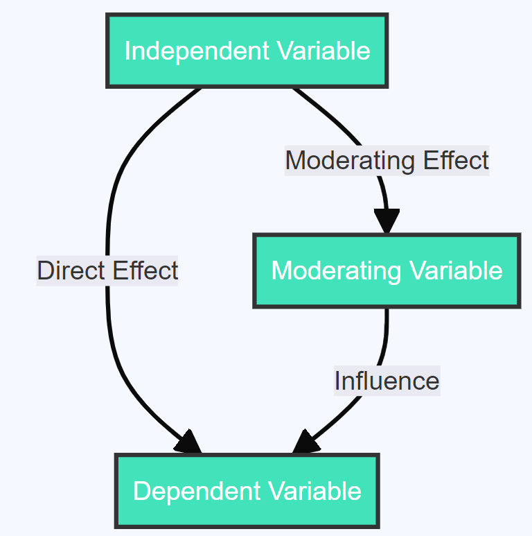
Of the three techniques I describe, moderation is probably the most tricky to understand. Essentially, it proposes that the size of a relationship between two variables changes depending upon the value of a third variable, known as a “moderator.” For example, in the diagram below you might find a simple main effect that is moderated by sex. That is, the relationship is stronger for women than for men:

With moderation, it is important to note that the moderating variable can be a category (e.g., sex) or it can be a continuous variable (e.g., scores on a personality questionnaire). When a moderator is continuous, usually you’re making statements like: “As the value of the moderator increases, the relationship between X and Y also increases.”

“Does X predict M, which in turn predicts Y?”

We might know that X leads to Y, but a mediation hypothesis proposes a mediating, or intervening variable. That is, X leads to M, which in turn leads to Y. In the diagram below I use a different way of visually representing things consistent with how people typically report things when using path analysis.

I use mediation a lot in my own research. For example, I’ve published data suggesting the relationship between perfectionism and depression is mediated by relationship conflict ( Mackinnon et al., 2012 ). That is, perfectionism leads to increased conflict, which in turn leads to heightened depression. Another way of saying this is that perfectionism has an indirect effect on depression through conflict.

Helpful links to get you started testing these hypotheses

Depending on the nature of your data, there are multiple ways to address each of these hypotheses using statistics. They can also be combined together (e.g., mediated moderation). Nonetheless, a core understanding of these three hypotheses and how to analyze them using statistics is essential for any researcher in the social or health sciences. Below are a few links that might help you get started:

Are you a little rusty with multiple regression? The basics of this technique are required for most common tests of these hypotheses. You might check out this guide as a helpful resource:

https://statistics.laerd.com/spss-tutorials/multiple-regression-using-spss-statistics.php

David Kenny’s Mediation Website provides an excellent overview of mediation and moderation for the beginner.

http://davidakenny.net/cm/mediate.htm

http://davidakenny.net/cm/moderation.htm

Preacher and Haye’s INDIRECT Macro is a great, easy way to implement mediation in SPSS software, and their MODPROBE macro is a useful tool for testing moderation.

http://afhayes.com/spss-sas-and-mplus-macros-and-code.html

If you want to graph the results of your moderation analyses, the excel calculators provided on Jeremy Dawson’s webpage are fantastic, easy-to-use tools:

http://www.jeremydawson.co.uk/slopes.htm

Tags mediation , moderation , regression , tutorial

37 replies on “The Three Most Common Types of Hypotheses”

I want to see clearly the three types of hypothesis

Thanks for your information. I really like this

Thank you so much, writing up my masters project now and wasn’t sure whether one of my variables was mediating or moderating….Much clearer now.

Thank you for simplified presentation. It is clearer to me now than ever before.

Thank you. Concise and clear

hello there

I would like to ask about mediation relationship: If I have three variables( X-M-Y)how many hypotheses should I write down? Should I have 2 or 3? In other words, should I have hypotheses for the mediating relationship? What about questions and objectives? Should be 3? Thank you.

Hi Osama. It’s really a stylistic thing. You could write it out as 3 separate hypotheses (X -> Y; X -> M; M -> Y) or you could just write out one mediation hypotheses “X will have an indirect effect on Y through M.” Usually, I’d write just the 1 because it conserves space, but either would be appropriate.

Hi Sean, according to the three steps model (Dudley, Benuzillo and Carrico, 2004; Pardo and Román, 2013)., we can test hypothesis of mediator variable in three steps: (X -> Y; X -> M; X and M -> Y). Then, we must use the Sobel test to make sure that the effect is significant after using the mediator variable.

Yes, but this is older advice. Best practice now is to calculate an indirect effect and use bootstrapping, rather than the causal steps approach and the more out-dated Sobel test. I’d recommend reading Hayes (2018) book for more info:

Hayes, A. F. (2018). Introduction to mediation, moderation, and conditional process analysis: A regression-based approach (2nd ed). Guilford Publications.

Hi! It’s been really helpful but I still don’t know how to formulate the hypothesis with my mediating variable.

I have one dependent variable DV which is formed by DV1 and DV2, then I have MV (mediating variable), and then 2 independent variables IV1, and IV2.

How many hypothesis should I write? I hope you can help me 🙂

Thank you so much!!

If I’m understanding you correctly, I guess 2 mediation hypotheses:

IV1 –> Med –> DV1&2 IV2 –> Med –> DV1&2

Thank you so much for your quick answer! ^^

Could you help me formulate my research question? English is not my mother language and I have trouble choosing the right words. My x = psychopathy y = aggression m = deficis in emotion recognition

thank you in advance

I have mediator and moderator how should I make my hypothesis

Can you have a negative partial effect? IV – M – DV. That is my M will have negative effect on the DV – e.g Social media usage (M) will partial negative mediate the relationship between father status (IV) and social connectedness (DV)?

Thanks in advance

Hi Ashley. Yes, this is possible, but often it means you have a condition known as “inconsistent mediation” which isn’t usually desirable. See this entry on David Kenny’s page:

Or look up “inconsistent mediation” in this reference:

MacKinnon, D. P., Fairchild, A. J., & Fritz, M. S. (2007). Mediation analysis. Annual Review of Psychology, 58, 593-614.

This is very interesting presentation. i love it.

This is very interesting and educative. I love it.

Hello, you mentioned that for the moderator, it changes the relationship between iv and dv depending on its strength. How would one describe a situation where if the iv is high iv and dv relationship is opposite from when iv is low. And then a 3rd variable maybe the moderator increases dv when iv is low and decreases dv when iv is high.

This isn’t problematic for moderation. Moderation just proposes that the magnitude of the relationship changes as levels of the moderator changes. If the sign flips, probably the original relationship was small. Sometimes people call this a “cross-over” effect, but really, it’s nothing special and can happen in any moderation analysis.

i want to use an independent variable as moderator after this i will have 3 independent variable and 1 dependent variable…. my confusion is do i need to have some past evidence of the X variable moderate the relationship of Y independent variable and Z dependent variable.

Dear Sean It is really helpful as my research model will use mediation. Because I still face difficulty in developing hyphothesis, can you give examples ? Thank you

Hi! is it possible to have all three pathways negative? My regression analysis showed significant negative relationships between x to y, x to m and m to y.

Hi, I have 1 independent variable, 1 dependent variable and 4 mediating variable May I know how many hypothesis should I develop?

Hello I have 4 IV , 1 mediating Variable and 1 DV

My model says that 4 IVs when mediated by 1MV leads to 1 Dv

Pls tell me how to set the hypothesis for mediation

Hi I have 4 IVs ,2 Mediating Variables , 1DV and 3 Outcomes (criterion variables).

Pls can u tell me how many hypotheses to set.

Thankyou in advance

I am in fact happy to read this webpage posts which carries tons of useful information, thanks for providing such data.

I see you don’t monetize savvystatistics.com, don’t waste your traffic, you can earn additional bucks every month with new monetization method. This is the best adsense alternative for any type of website (they approve all websites), for more info simply search in gooogle: murgrabia’s tools

what if the hypothesis and moderator significant in regrestion and insgificant in moderation?

Thank you so much!! Your slide on the mediator variable let me understand!

Very informative material. The author has used very clear language and I would recommend this for any student of research/

Hi Sean, thanks for the nice material. I have a question: for the second type of hypothesis, you state “That is, the relationship is stronger for men than for women”. Based on the illustration, wouldn’t the opposite be true?

Yes, your right! I updated the post to fix the typo, thank you!

I have 3 independent variable one mediator and 2 dependant variable how many hypothesis I have 2 write?

Sounds like 6 mediation hypotheses total:

X1 -> M -> Y1 X2 -> M -> Y1 X3 -> M -> Y1 X1 -> M -> Y2 X2 -> M -> Y2 X3 -> M -> Y2

Clear explanation! Thanks!

What is a Moderating Variable? Definition & Example

A moderating variable is a type of variable that affects the relationship between a dependent variable and an independent variable .

When performing regression analysis , we’re often interested in understanding how changes in an independent variable affect a dependent variable. However, sometimes a moderating variable can affect this relationship.

For example, suppose we want to fit a regression model in which we use the independent variable hours spent exercising each week to predict the dependent variable resting heart rate .

We suspect that more hours spent exercising is associated with a lower resting heart rate. However, this relationship could be affected by a moderating variable such as gender .

It’s possible that each extra hour of exercise causes resting heart rate to drop more for men compared to women.

Another example of a moderating variable could be age . It’s likely that each extra hour of exercise causes resting heart rate to drop more for younger people compared to older people.

Properties of Moderating Variables

Moderating variables have the following properties:

1. Moderating variables can be qualitative or quantitative .

Qualitative variables are variables that take on names or labels. Examples include:

Gender (Male or Female)
Education Level (High School Degree, Bachelor’s Degree, Master’s Degree, etc.)
Marital Status (Single, Married, Divorced)

Quantitative variables are variables that take on numerical values. Examples include:

Square Footage
Population Size

In the previous examples, gender was a qualitative variable that could affect the relationship between hours studied and resting heart rate while age was a quantitative variable that could potentially affect the relationship.

2. Moderating variables can affect the relationship between an independent and dependent variable in a variety of ways.

Moderating variables can have the following effects:

Strengthen the relationship between two variables.
Weaken the relationship between two variables.
Negate the relationship between two variables.

Depending on the situation, a moderating variable can moderate the relationship between two variables in many different ways.

How to Test for Moderating Variables

If X is an independent variable (sometimes called a “predictor” variable) and Y is a dependent variable (sometimes called a “response” variable), then we could write a regression equation to describe the relationship between the two variables as follows:

Y = β 0 + β 1 X

If we suspect that some other variable, Z , is a moderator variable, then we could fit the following regression model:

Y = β 0 + β 1 X 1 + β 2 Z + β 3 XZ

In this equation, the term XZ is known as an interaction term .

If the p-value for the coefficient of XZ in the regression output is statistically significant, then this indicates that there is a significant interaction between X and Z and Z should be included in the regression model as a moderator variable.

We would write the final model as:

Y = β 0 + β 1 X + β 2 Z + β 3 XZ

If the p-value for the coefficient of XZ in the regression output is not statistically significant, then Z is not a moderator variable.

However it’s possible that the coefficient for Z could still be statistically significant. In this case, we would simply include Z as another independent variable in the regression model.

We would then write the final model as:

Y = β 0 + β 1 X + β 2 Z

Additional Resources

How to Read and Interpret a Regression Table How to Use Dummy Variables in Regression Analysis Introduction to Confounding Variables

Featured Posts

Hey there. My name is Zach Bobbitt. I have a Masters of Science degree in Applied Statistics and I’ve worked on machine learning algorithms for professional businesses in both healthcare and retail. I’m passionate about statistics, machine learning, and data visualization and I created Statology to be a resource for both students and teachers alike. My goal with this site is to help you learn statistics through using simple terms, plenty of real-world examples, and helpful illustrations.

One Reply to “What is a Moderating Variable? Definition & Example”

Nicely explained Moderation concept.

Moderating Variables in Research: A Comprehensive Guide with Real-World Examples

Welcome to the intriguing world of research, where even the simplest of studies can hide complex layers of interaction and causality. In today’s exploration, we’re delving into the fascinating domain of moderating variables . Buckle up, as we’re about to take an intellectual detour through the heart of research methods, enriched with practical examples to fortify your understanding.

Statssy.com is your trusted guide in this journey, as we continually aim to illuminate the fundamental and advanced concepts of data analytics, research methods, and machine learning.

The Trio of Research: Independent, Dependent, and Moderating Variables

Before we dive into the nuances of moderating variables, let’s familiarize ourselves with the foundational components of any research study: the Independent Variable (IV), the Dependent Variable (DV), and, of course, the Moderating Variable (MV). These components serve as the building blocks of any research design, each having a unique and crucial role.

Independent Variable (IV) : This is the experimental lever, the factor manipulated or changed by the researchers in a study. It’s the variable that stands on its own – ‘independent’ by definition. Dependent Variable (DV) : As the name suggests, this variable ‘depends’ on the independent variable. It represents the outcome or result that researchers aim to measure and is influenced by the changes in the IV. Moderating Variable (MV) : The dark horse of our trio, the moderating variable affects the strength or direction of the relationship between the IV and DV. In simpler terms, it modifies the impact of the independent variable on the dependent variable. This intriguing interaction is what we will explore today.

Understanding this triad sets the foundation for grasping the nuances of moderating variables. So, with the stage set, let’s proceed to explore the world of moderating variables with vivid examples.

Need Help in Your Research?

Schedule a Call

Diving into moderating variables: examples unveiled.

Illustrations make understanding easier, and when we talk about moderating variables, they become all the more important. They help us visualize how these variables weave themselves into the fabric of a study, subtly influencing the relationship between the IV and DV. Let’s explore some real-world examples:

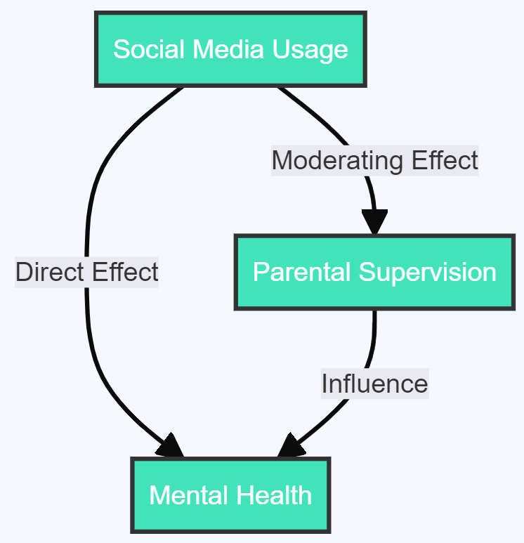
Parental Supervision moderating the effect of Social Media Usage on Mental Health : In this case, the extent of parental supervision might moderate (either decrease or increase) the impact of social media usage on a child’s mental health. In a nutshell, the moderating variable is an intriguing character, influencing the relationship between two other variables in a study. It may affect the intensity, direction, or even the very nature of this relationship, making it a crucial factor to consider in research design.

With this introduction, we’ve just begun our deep dive into the fascinating realm of moderating variables. Stick with us as we continue our exploration, further unraveling the layers of this complex yet fascinating component of research.

The Power of Moderating Variables: More Examples

Let’s carry on with our journey into the realm of moderating variables, further solidifying our understanding through a broader range of examples:

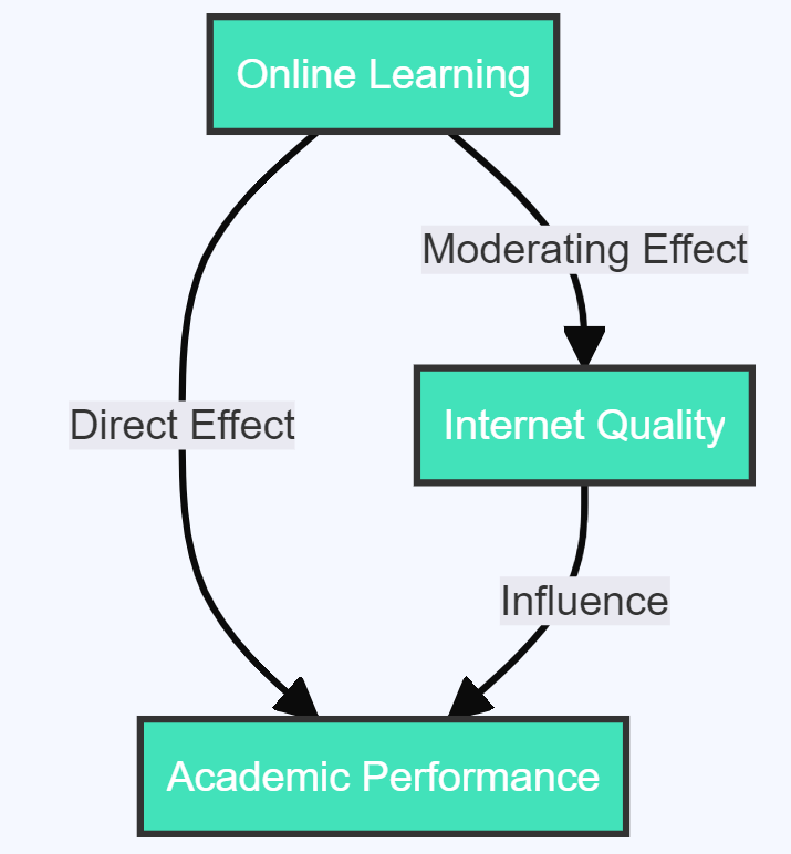
Internet Quality moderating the effect of Online Learning on Academic Performance : Here, the quality of the internet could determine the extent of the impact of online learning on academic performance. In regions with high-speed internet, the impact might be positive, whereas, in regions with poor internet connectivity, the impact might be negative.

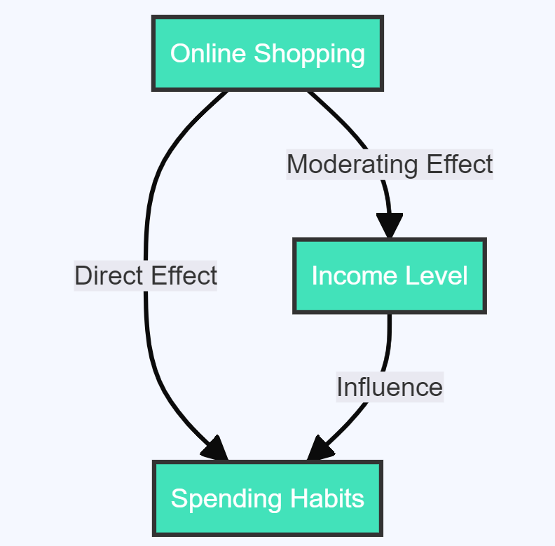
Income Level moderating the effect of Online Shopping on Spending Habits : The level of income could influence how online shopping impacts a person’s spending habits. For instance, high-income individuals may splurge more when shopping online, whereas low-income individuals might show more restraint.

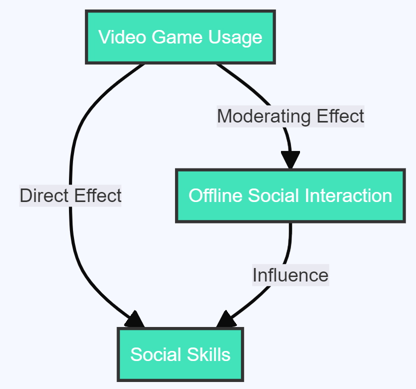
Offline Social Interaction moderating the effect of Video Game Usage on Social Skills : In this case, the amount of offline social interaction could temper the influence of video game usage on social skills. For those who also engage in a healthy amount of offline social activities, the impact might be negligible, but for those who primarily interact socially via video games, the impact might be more pronounced.

These examples illuminate the multidimensional impact a moderating variable can have on a research study, providing a more nuanced understanding of the subject matter under investigation.

Harnessing the Influence: The Significance of Moderating Variables

You may be wondering, why are moderating variables so important in research? Can’t we simply analyze the direct relationship between the independent and dependent variables?

Well, in an ideal world, where every cause has a single, predictable effect, that might be possible. But the real world is full of complexities and interdependencies, which is where the moderating variable steps in.

A moderating variable helps us better understand the ‘how’ and ‘when’ of the relationship between the IV and DV. It reveals under what conditions the IV has an effect on the DV, and the nature of this effect.

This ability to bring forth the conditional effects in a study is what makes moderating variables a critical tool in research design. They allow us to examine relationships that are more dynamic, more reflective of the world’s complexity, ultimately leading us to more nuanced and accurate findings.

However, as with any tool, the key to harnessing the power of moderating variables lies in understanding their application and interpretation, which we will delve into in our upcoming sections.

Navigating Through the Sea of Examples: More Explorations

The power of moderating variables can be further revealed as we delve into even more examples:

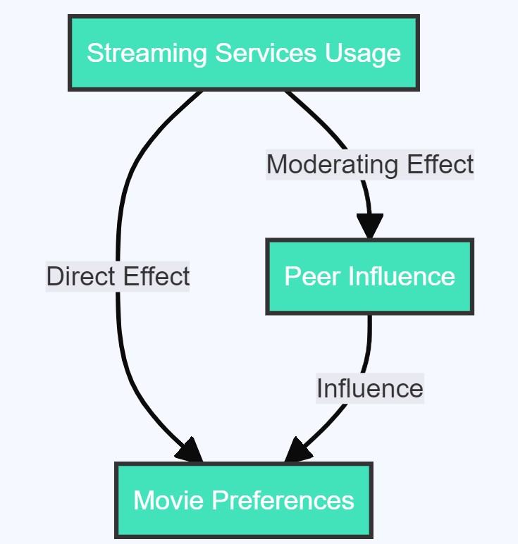
Peer Influence moderating the effect of Streaming Services Usage on Movie Preferences : The influence of peers could mitigate or intensify the impact of streaming service usage on movie preferences. For those with highly influential peers, their movie choices might be more determined by their friends, irrespective of what they watch on streaming platforms. On the other hand, those with less influential peers might rely more on their streaming history when selecting movies.

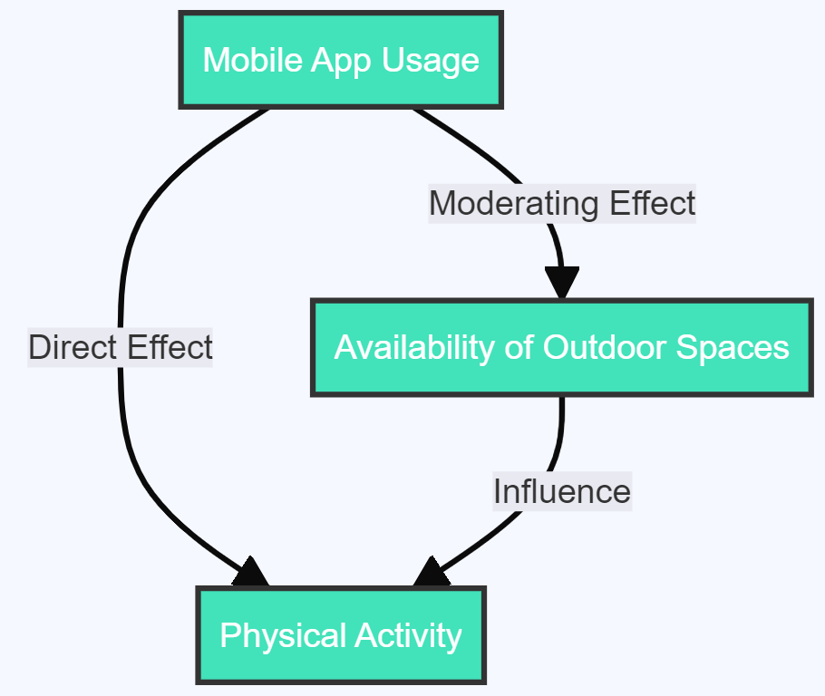
Availability of Outdoor Spaces moderating the effect of Mobile App Usage on Physical Activity : The presence of accessible outdoor spaces could determine how mobile app usage affects physical activity. People who live in areas with ample outdoor spaces might use certain apps without affecting their level of physical activity, while those in more congested urban areas might exhibit reduced physical activity with increased mobile app usage.

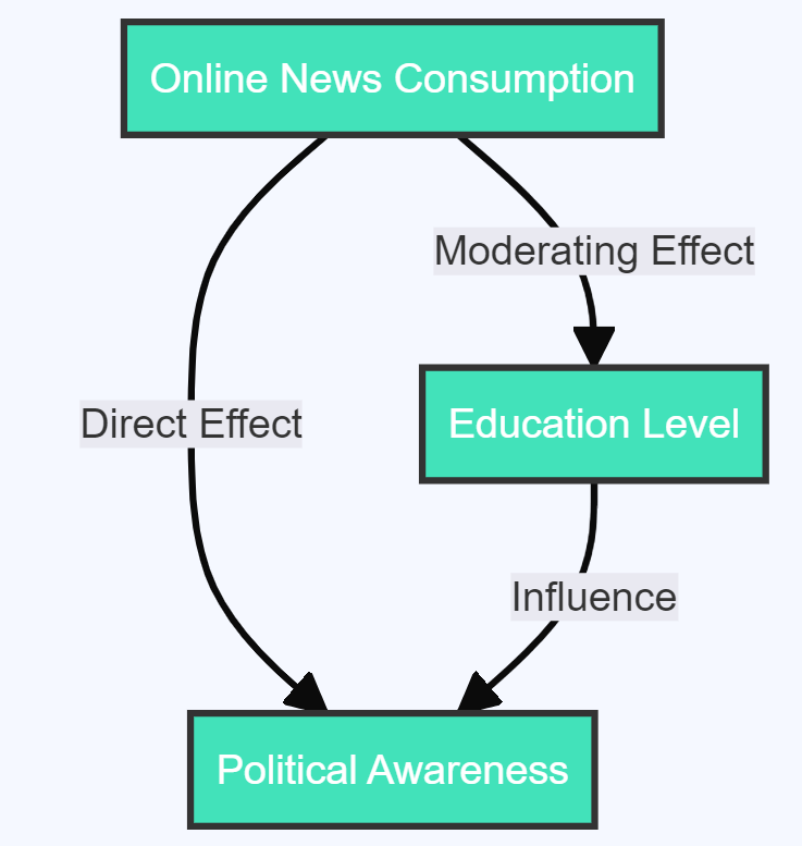
Education Level moderating the effect of Online News Consumption on Political Awareness : A person’s education level could affect how online news consumption influences their political awareness. Those with higher education levels may extract more insightful information and exhibit increased political awareness with more online news consumption, whereas the less educated might not see a significant change in their political awareness.

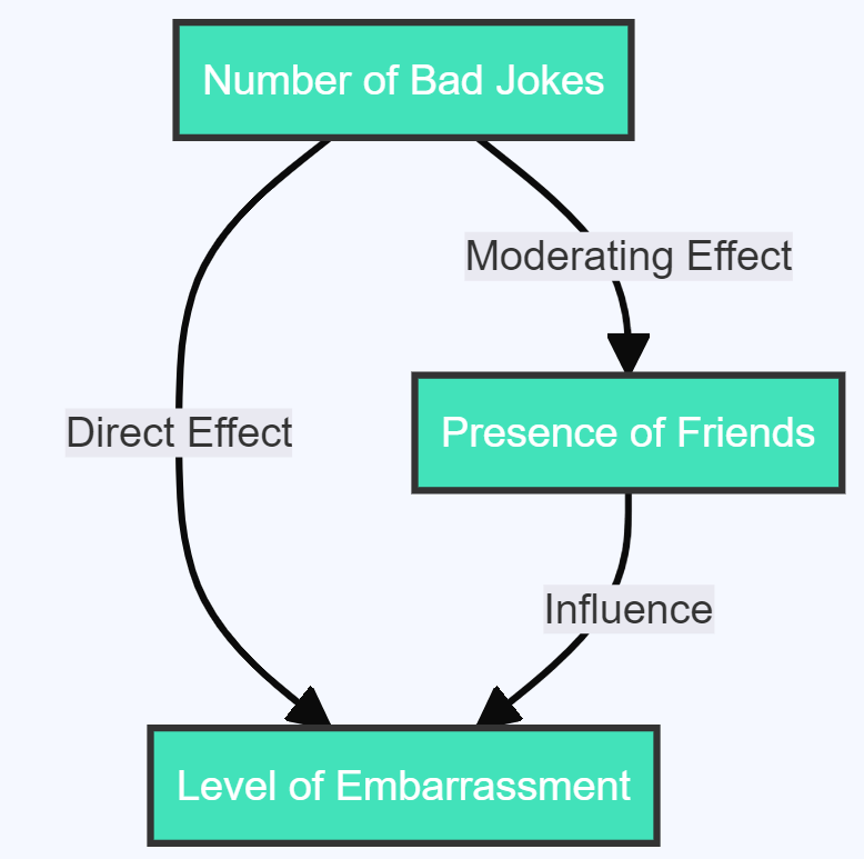
Presence of Friends moderating the effect of Number of bad Jokes Told on Level of Embarrassment : The presence of friends may decrease or increase the level of embarrassment felt when a person tells a certain number of bad jokes. It depends on the relationship dynamics within the group – are the friends supportive and likely to laugh along, or are they more likely to mock the joke-teller?

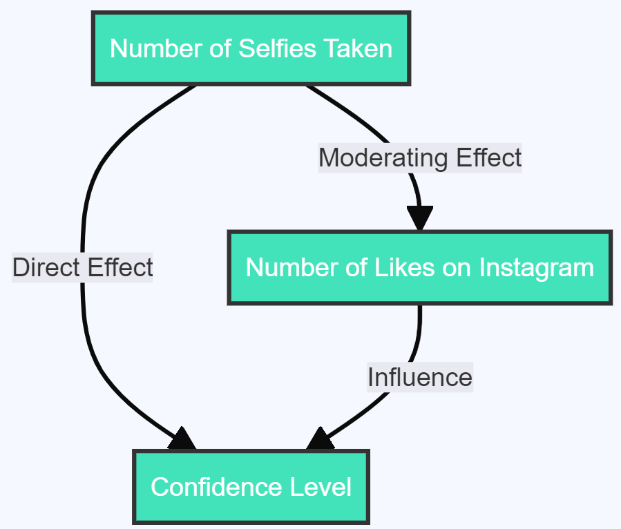
Number of Likes on Instagram moderating the effect of Number of Selfies Taken on Confidence Level : The number of selfies taken can affect confidence, but the impact is likely to vary depending on the number of likes received on Instagram. More likes can lead to increased confidence, while fewer likes might lower it, despite the number of selfies taken.

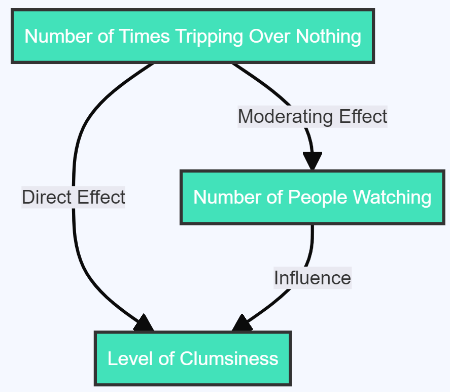
Number of People Watching moderating the effect of Number of Times Tripping Over Nothing on Level of Clumsiness : The more people are watching, the more clumsy a person might feel if they trip over nothing multiple times. With fewer spectators, the perceived level of clumsiness might be less.

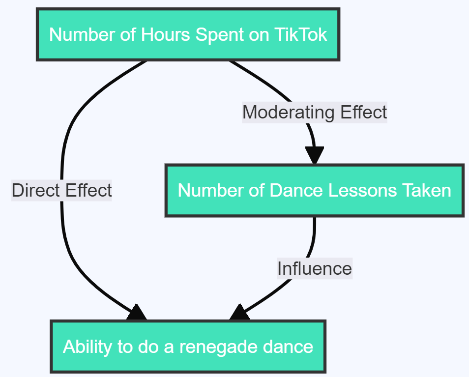
Number of Dance Lessons Taken moderating the effect of Number of Hours Spent on TikTok on Ability to Do a Renegade Dance : More dance lessons can enhance the ability to do a Renegade Dance, even if the number of hours spent on TikTok is high. Conversely, fewer dance lessons might not improve the dance skills despite many hours spent watching TikTok.

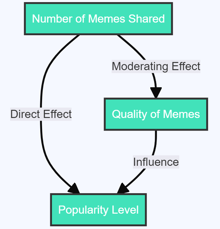
Quality of Memes moderating the effect of Number of Memes Shared on Popularity Level : Sharing a large number of memes may not necessarily increase popularity if the quality of those memes is low. High-quality memes can boost popularity, even when the quantity shared is less.

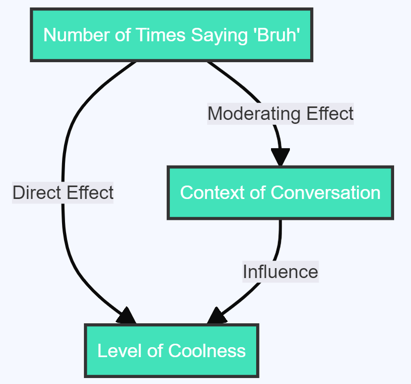
Context of Conversation moderating the effect of Number of Times Saying ‘Bruh’ on Level of Coolness : Saying ‘Bruh’ multiple times might be seen as cool in a casual conversation among peers. However, the same might not be considered cool in a formal or serious conversation. Thus, the context moderates the effect of the frequency of saying ‘Bruh’ on perceived coolness.

These instances further elucidate how the moderating variable can contextualize and refine our understanding of the relationship between an independent and a dependent variable.

Identifying Moderating Variables: The Vital Steps

After gaining a robust understanding of what a moderating variable is and how it operates, let’s move onto identifying them in research studies. Here are the crucial steps to follow:

Formulate the Research Question : The research question should be clear and concise, and it should mention the presumed moderating variable.
Design the Study : Design your research such that it enables the isolation of the moderating variable.
Collect Data : Gather data on the independent, dependent, and moderating variables. It’s essential to measure all three for the subsequent analysis.
Analyze the Data : Use statistical methods to analyze the data and ascertain the impact of the moderating variable.

Remember, correctly identifying and incorporating moderating variables into your study can significantly enhance its depth, richness, and overall validity. But keep an eye out! Misidentification or misuse can lead to misleading conclusions.

In the next section, we’ll explore the potential challenges and common pitfalls to avoid when dealing with moderating variables.

Potential Pitfalls and Challenges: A Guided Cautionary Tale

Engaging with moderating variables can feel like navigating a labyrinth at times. Missteps could potentially distort your research findings. Here are some of the most common pitfalls and challenges you should keep an eye on:

Misidentification : An all-too-common mistake is misidentifying a moderating variable as either an independent or a dependent variable. Understanding and defining the role of each variable in your study will help mitigate this risk.
Multicollinearity : This phenomenon arises when your independent variables are too closely associated with each other. It can result in unstable estimates of regression coefficients, making it hard to interpret your results. Multicollinearity can be particularly challenging when it involves your moderating variable.
Overfitting : Trying to fit too many moderating variables into your model can lead to overfitting, where your model performs well on the training data but poorly with new, unseen data. Striking a balance is key here.
Misinterpretation : Even if correctly identified and measured, moderating variables can still be misinterpreted. Researchers must ensure they accurately interpret the impact of the moderating variable on the relationship between the independent and dependent variables.

Understanding these challenges is crucial, but it’s only one side of the coin. The next step is learning how to correctly interpret and present the results involving moderating variables.

Making Sense of Results: The Art of Interpretation

Interpreting results involving moderating variables can be a complex task. However, by following a structured approach, it becomes more manageable:

Analysis : Use appropriate statistical methods to analyze your data, such as regression analysis or Analysis of Variance (ANOVA).
Visualisation : Plotting the interaction between your variables can often make it easier to understand. Interaction plots or 3D surface plots are commonly used.
Interpretation : Consider the direction and magnitude of the effect of your moderating variable. Does it strengthen or weaken the relationship between your independent and dependent variables? Does it reverse the relationship?
Communication : Explain the role of your moderating variable in layman’s terms. Your research should be accessible to those outside of your specific field.

In the final segment of this comprehensive guide, we will wrap up our discussion and reinforce some key takeaways about moderating variables.

Wrapping Up: Final Thoughts on Moderating Variables

A researcher’s journey into the world of moderating variables can be complex and, at times, even challenging. Still, it’s an essential path to tread for those seeking to unveil nuanced and contextual understanding from their research. It is the subtle interplay of variables that often delivers the most valuable insights.

But let’s not forget the individuals who are at the heart of this journey – the researchers. To those who are keen on incorporating moderating variables in their research, here’s a distilled summary of the key takeaways from this guide:

Aim for Clarity : Understand and clearly define the role of each variable in your study. The success of your research hinges on how well you’ve comprehended the triad of independent, dependent, and moderating variables.
Design Matters : Structure your study keeping the moderating variable(s) in mind. Be wary of common pitfalls, like multicollinearity and overfitting.
Statistical Tools are your Friends : Familiarise yourself with the statistical tools necessary to analyze the effects of your moderating variable(s).
Interpretation is Key : Ensure that you interpret the results correctly. Remember, the effectiveness of your research lies in its interpretation.
Communicate with Precision : Lastly, communicate your findings effectively. The world needs to know what you’ve discovered.

Embarking on a research journey with moderating variables in tow might be challenging, but the result is undeniably rewarding. The added depth and context they bring to your research can be the difference between a good study and a great one.

Happy researching!

We trust that this article has provided you with a deep understanding of the topic. Feel free to reach out for any further queries or discussions. Keep visiting statssy.com for more insights and guides on data analytics, research methods, and machine learning.

Submit a Comment Cancel reply

Your email address will not be published. Required fields are marked *

Save my name, email, and website in this browser for the next time I comment.

Please wait..
Into 2023: The Best Must-Attend Data Science Conferences You Can’t Miss! 🚀
Power of Data Analysis in Research: A Comprehensive Guide to Types, Methods, and Tools
Becoming a Data Analyst After B. Com: A Comprehensive Roadmap

Unlock the power of data with our user-friendly statistics calculator.

Explore our data science courses to supercharge your career growth in the world of data and analytics.

Test Your Skills With Our Quiz

Contact me today i have solution to all your problems..

Home » Moderating Variable – Definition, Analysis Methods and Examples

Moderating Variable – Definition, Analysis Methods and Examples

Table of Contents

Moderating Variable

Definition:

A moderating variable is a variable that affects the strength or direction of the relationship between two other variables. It is also referred to as an interactive variable or a moderator.

In social science research, a moderating variable is often used to understand how the relationship between two variables changes depending on the level of a third variable. For example, in a study examining the relationship between stress and job performance, age might be a moderating variable. The relationship between stress and job performance may be stronger for younger workers than for older workers, meaning that age is influencing the relationship between stress and job performance.

Moderating Variable Analysis Methods

Moderating Variable Analysis Methods are as follows:

Regression Analysis

Regression analysis is a statistical technique that examines the relationship between a dependent variable and one or more independent variables. In the case of a moderating variable, a regression analysis can be used to examine the interaction between the independent and moderating variables in predicting the dependent variable. This can be done using a simple regression or multiple regression analysis, depending on the number of variables involved.

Analysis of Variance (ANOVA)

ANOVA is a statistical method used to compare the means of two or more groups. In the case of a moderating variable, ANOVA can be used to compare the mean differences between groups based on different levels of the moderating variable. For example, if age is a moderating variable, ANOVA can be used to compare the mean differences in job performance between younger and older workers at different levels of stress.

Multiple Regression Analysis

Multiple regression analysis is a statistical technique used to predict the value of a dependent variable based on two or more independent variables. In the case of a moderating variable, multiple regression analysis can be used to examine the interaction between the independent variables and the moderating variable in predicting the dependent variable.

Moderating Variable Examples

Here are a few examples of moderating variables:

Age as a moderating variable : Suppose a study examines the relationship between exercise and heart health. Age may act as a moderating variable, influencing the relationship between exercise and heart health. For example, the relationship between exercise and heart health may be stronger for younger adults compared to older adults.
Gender as a moderating variable: Consider a study examining the relationship between salary and job satisfaction. Gender may act as a moderating variable, influencing the relationship between salary and job satisfaction. For example, the relationship between salary and job satisfaction may be stronger for men than for women.
Social support as a moderating variable: Suppose a study examines the relationship between stress and mental health. Social support may act as a moderating variable, influencing the relationship between stress and mental health. For example, the relationship between stress and mental health may be stronger for individuals with low social support compared to those with high social support.
Education level as a moderating variable: Consider a study examining the relationship between technology use and academic performance. Education level may act as a moderating variable, influencing the relationship between technology use and academic performance. For example, the relationship between technology use and academic performance may be stronger for individuals with higher education levels compared to those with lower education levels.

Applications of Moderating Variable

Market research: Moderating variables are often used in market research to identify the factors that influence consumer behavior. For example, age, income, and education level can be moderating variables that affect the relationship between advertising and consumer purchasing behavior.
Psychology : In psychology, moderating variables can help explain the relationship between variables such as personality traits and job performance. For example, a person’s level of conscientiousness may moderate the relationship between their job performance and job satisfaction.
Education: In education, moderating variables can help explain the relationship between teaching methods and student learning outcomes. For example, the level of student engagement may moderate the relationship between a teacher’s teaching style and student learning outcomes.
Health : In health research, moderating variables can help explain the relationship between risk factors and health outcomes. For example, gender may moderate the relationship between smoking and lung cancer.
Social sciences: In the social sciences, moderating variables can help explain the relationship between variables such as income and happiness. For example, the level of social support may moderate the relationship between income and happiness.

Purpose of Moderating Variable

The purpose of a moderating variable is to identify the conditions under which the relationship between two other variables changes or becomes stronger or weaker. In other words, a moderating variable helps to explain the context in which a particular relationship exists.

For example, let’s consider the relationship between stress and job performance. The relationship may be different depending on the level of social support that an individual receives. In this case, social support is the moderating variable. If an individual has high levels of social support, the negative impact of stress on job performance may be reduced. On the other hand, if an individual has low levels of social support, the negative impact of stress on job performance may be amplified.

The purpose of identifying moderating variables is to help researchers better understand the complex relationships between variables and to provide more accurate predictions of outcomes in specific situations. By identifying the conditions under which a relationship exists or changes, researchers can develop more effective interventions and treatments. Moderating variables can also help to identify subgroups of individuals who may benefit more or less from a particular intervention or treatment.

When to use Moderating Variable

Here are some scenarios where using a moderating variable can be helpful:

When there is a complex relationship: In situations where the relationship between two variables is complex, a moderating variable can help to clarify the relationship. For example, the relationship between stress and job performance may be influenced by a variety of factors such as job demands, social support, and coping mechanisms.
When there is a subgroup effect : In situations where the effect of one variable on another is stronger or weaker for certain subgroups of individuals, a moderating variable can be helpful. For example, the relationship between exercise and weight loss may be stronger for individuals who are obese compared to individuals who are not obese.
When there is a need for tailored interventions: In situations where the effect of one variable on another is different for different individuals, a moderating variable can be useful for developing tailored interventions. For example, the relationship between diet and weight loss may be influenced by individual differences in genetics, metabolism, and lifestyle.

Characteristics of Moderating Variable

The following are some key characteristics of moderating variables:

Interact with other variables : Moderating variables interact with other variables in a statistical relationship, influencing the strength or direction of the relationship between two other variables.
Independent variable: Moderating variables are independent variables in a statistical analysis, meaning that they are not influenced by any of the other variables in the analysis.
Categorical or continuous: Moderating variables can be either categorical or continuous. Categorical moderating variables have distinct categories or levels (e.g., gender), while continuous moderating variables can take on any value within a range (e.g., age).
Can be identified through statistical analysis: Moderating variables can be identified through statistical analysis using regression analysis or ANOVA. Researchers can examine the interaction between the independent and moderating variables in predicting the dependent variable to determine if the moderating variable has a significant impact.
Influence the relationship between other variables : The impact of a moderating variable on the relationship between other variables can be positive, negative, or null. It depends on the specific research question and the data analyzed.
Provide insight into underlying mechanisms: Moderating variables can provide insight into underlying mechanisms driving the relationship between other variables, providing a more nuanced understanding of the relationship.

Advantages of Moderating Variable

There are several advantages of using a moderating variable in research:

Provides a more nuanced understanding of relationships: By identifying the conditions under which a particular relationship exists or changes, a moderating variable provides a more nuanced understanding of the relationship between two variables. This can help researchers to better understand complex relationships and to develop more effective interventions.
Improves accuracy of predictions: By identifying the conditions under which a relationship exists or changes, a moderating variable can improve the accuracy of predictions about outcomes in specific situations. This can help researchers to develop more effective interventions and treatments.
Identifies subgroups of individuals : Moderating variables can help to identify subgroups of individuals who may benefit more or less from a particular intervention or treatment. This can help researchers to develop more tailored interventions that are more effective for specific groups of individuals.
Increases generalizability: By identifying the conditions under which a relationship exists or changes, a moderating variable can increase the generalizability of findings. This can help researchers to apply findings from one study to other populations and contexts.
Provides more complete understanding of phenomena : By considering the role of a moderating variable, researchers can gain a more complete understanding of the phenomena they are studying. This can help to identify areas for future research and to generate new hypotheses.

Disadvantages of Moderating Variable

Disadvantages of Moderating Variable are as follows:

Complexity: The use of moderating variables can make research more complex and challenging to design, analyze, and interpret. This can require more resources and expertise than simpler research designs.
Increased risk of Type I errors : When using a moderating variable, there is an increased risk of Type I errors, or false positives. This can occur when a relationship is identified that appears significant, but is actually due to chance.
Reduced generalizability: Moderating variables can limit the generalizability of findings to other populations and contexts. This is because the relationship between two variables may be influenced by different moderating variables in different contexts.
Limited explanatory power: While moderating variables can help to identify conditions under which a relationship exists, they may not provide a complete explanation of why the relationship exists. Other variables may also play a role in the relationship.
Data requirements: Using moderating variables often requires larger sample sizes and more data than simpler research designs. This can increase the time and resources required to conduct the research.

About the author

Muhammad Hassan

Researcher, Academic Writer, Web developer

Control Variable – Definition, Types and Examples

Qualitative Variable – Types and Examples

Variables in Research – Definition, Types and...

Categorical Variable – Definition, Types and...

Independent Variable – Definition, Types and...

Ratio Variable – Definition, Purpose and Examples

Utility Menu

Arts, Science and Writing Studio

A place for everyone to share and learn.

Regression with a moderator 101

What is a moderator?

The linear regression modeling as illustrated in chapter 3 has different variations, just like ANOVA. The mathematics behind various regression models can be messy; however, the main objective of this book is to how to apply it. Regression with a moderator is an advance regression model to test for interaction, but what is a moderator in the first place?

A moderator was defined in Hayes (2017), “The effect of X on some variable Y is moderated by W if its size, sign, or strength depends on or can be predicted by W. In that case, W is said to be a moderator of X’s effect on Y, or that W and X interact in their influence on Y (220).” Now, let’s translate it into English. Let’s consider the following hypothetical scenarios.

You live in a city A or a literally utopian city with extremely low crime rate. Everyone in the city has abundant resources. There are many designer shops including Gucci, Louis Vuitton, Montblanc, etc. In the city, people with higher income tend to buy designer products to exhibit their socioeconomic status.

Now, it is reasonable to assume there is a positive significant correlation between the income and the amount of money spent on designer products. Let’s assume that beta is 20, and p-value is .01.

You live in a city B town where the crime rate has been skyrocketing in the past decade. Everyone in the city is afraid of being robbed. Therefore, designer shops are not quite as popular as they are in the miracle town. In city B, people with higher income do not really buy designer products to exhibit their socioeconomic status. Instead, they hire personal guards or install high-tech security system at home.

Now, consider the correlation between the income and the money spent on designer products. It vanishes. There is no significant correlation anymore. Let’s assume that beta is .02, and p-value is .82.

If you were a researcher, you collect samples from both city A and B. Your research population is residents from both city A and B, and you found that income is not a significant predictor variable of the money spent on designer products. Is your finding accurate? The answer is obvious NO. What is happening here? What makes the difference?

The main difference between city A and B is the crime rate. The crime rate influences people’s perception of safety, or how safe people think it is to exhibit their wealth by wearing designer products. People’s perception of safety here is a moderator. Put it back to the definition. People’s perception about safety is a moderator of income’s effect on the amount of money they spend on designer products, or people’s perception of safe and their income interacts with the amount of money they spend on designer products.

The other way to think how a moderator works is to look at beta or coefficient. In the first scenario when the moderator’s size is high, meaning that people have a high sense of security, the corresponding coefficient is 20. When the moderator’s size is low, meaning that people have a low sense of security, the corresponding coefficient is 0.02 which is a lot lower.

Figure 5.1.a Illustrating the moderator

Look at the figure 5.1.a, the moderator variable is color-coded by blue and orange. Both lines are the linear regression line where income predicts the money spent on designer products. The orange one is in the dangerous city where people do not feel safe showing off their designer products while the blue one is in the safe city where people feel safe doing so. It is logically plausible.

Regression with a moderator?

What is the statistical way to test for an interaction? How can we test if there is a significant moderator? First, we need to think if it logically makes sense. When one variable can change the direction of another variable, it is a potential candidate for the moderator.

Let’s consider the following hypothesis. Students tend to develop a more positive attitude towards the renewable energy policy if he/she knows more about climate change. Assume that we do not find a correlation between attitude towards the renewable energy policy and the amount of knowledge about climate change. We can stop here concluding that the data does not support enough evidences to reject the null.

If we do not know anything about moderators, we would definitely stop here, but since we know the concept of the moderator. Maybe, political stand or belief about climate change might be a moderator. If a person believes that climate change is fake and created as a political tool by the leftist, it is possible that he would only read and accumulate knowledge about why climate change is fake due to the conformation bias. Therefore, climate change deniers might indeed spend more time reading and have a great volume of knowledge about the invalidity of climate change. Therefore, for people holding this belief, there might be a negative correlation instead of a positive correlation. In fact, then, if tested to be significant, the belief about whether climate change is real is the moderator here!

The formula for regression with a moderator is

Y= b 1 X 1 + b 2 X 2 + b 3 X 1 X 2 +C (5.1)

By testing this model, three possible coefficients and p values would be given. Then, b1 and b2 is the coefficient for direct effect while B3 is the interaction. P value for b3 would indicate whether the correlation is significant.

Applying to Gender Report Data

Are there any interaction in the World Bank Gender Report Database (2017)? Off course, there are. Let’s look at one closer. Let’s define binary qualitative variable X (independent variable) to be whether law requires equal gender hiring (1=yes; 0=no). Then, define a quantitative continuous variable Y (dependent variable) to be expected years of schooling for girls in the country. Now, we define our moderator M to be whether men and married women have equal ownership rights to property.

Our research hypothesis is legislation about whether men and married women, and legislation about whether law requires equal gender hiring interacts in their influence to expected years of schooling for girls in a country.

The result is significant. Let’s take a look at the figure 5.1 (b).

Figure 5.1(b)

It is obvious that marriage with or without equal ownership of property changes the coefficient. For countries with legislation requiring equal ownership within marriage, there is a positive correlation between law requiring equal gender hiring and expected years of schooling for girls. It means that girls receive longer education if the countries have laws requiring equal gender hiring.

However, if the countries do not have legislation requiring equal ownership, there is a negative correlation meaning girls receive less education if the countries have laws requiring equal gender hiring. It is plausible logically. If there is no hope for females because once they are married, their husbands own everything, there is no point for them to go to school even if there is law requiring equal gender hiring. Why even work if all money females make belong to their husbands.

To run regression with a moderator, you can either code the moderator by multiplying your independent variable and moderator. Otherwise, you can use Andrew F. Hayes’s process in SPSS. It also gives you conditional effects of the focal predictor at values of the moderator. Please read Andrew F. Hayes’s book, Introduction to Mediation, Moderation, and Conditional Process Analysis , if you want to learn more about moderation and conditional process analysis.

The interaction modeling can help us explain a lot of real-life scenarios. Sometimes, even if two variables are not correlated significant, there would still something to discover.

Practice and Homework

Hayes, A. F. (2017). Introduction to Mediation, Moderation, and Conditional Process Analysis, Second Edition: A Regression-Based Approach. Guilford Publications.

Call for Authors and Research Methodologists
Let's Run Some Analysis
Theory of Reverse Interest

Scientific research methods are not just for PhD. In fact, you can learn how to apply scientific methods and statistical tests in no time! The Research Methods and Statistics section will help you learn some statistical tests which are commonly used in scientific research. The goal is to explain the materials without 0 calculus involved, and we will make it as practical and easy as possble.

With scientific methods, you will never have to rely on getting information from media anymore. You can discover the truth with your own hands!

Have a language expert improve your writing

Run a free plagiarism check in 10 minutes, automatically generate references for free.

Knowledge Base
Methodology
How to Write a Strong Hypothesis | Guide & Examples

How to Write a Strong Hypothesis | Guide & Examples

Published on 6 May 2022 by Shona McCombes .

A hypothesis is a statement that can be tested by scientific research. If you want to test a relationship between two or more variables, you need to write hypotheses before you start your experiment or data collection.

What is a hypothesis, developing a hypothesis (with example), hypothesis examples, frequently asked questions about writing hypotheses.

A hypothesis states your predictions about what your research will find. It is a tentative answer to your research question that has not yet been tested. For some research projects, you might have to write several hypotheses that address different aspects of your research question.

A hypothesis is not just a guess – it should be based on existing theories and knowledge. It also has to be testable, which means you can support or refute it through scientific research methods (such as experiments, observations, and statistical analysis of data).

Variables in hypotheses

Hypotheses propose a relationship between two or more variables . An independent variable is something the researcher changes or controls. A dependent variable is something the researcher observes and measures.

In this example, the independent variable is exposure to the sun – the assumed cause . The dependent variable is the level of happiness – the assumed effect .

Prevent plagiarism, run a free check.

Step 1: ask a question.

Writing a hypothesis begins with a research question that you want to answer. The question should be focused, specific, and researchable within the constraints of your project.

Step 2: Do some preliminary research

Your initial answer to the question should be based on what is already known about the topic. Look for theories and previous studies to help you form educated assumptions about what your research will find.

At this stage, you might construct a conceptual framework to identify which variables you will study and what you think the relationships are between them. Sometimes, you’ll have to operationalise more complex constructs.

Step 3: Formulate your hypothesis

Now you should have some idea of what you expect to find. Write your initial answer to the question in a clear, concise sentence.

Step 4: Refine your hypothesis

You need to make sure your hypothesis is specific and testable. There are various ways of phrasing a hypothesis, but all the terms you use should have clear definitions, and the hypothesis should contain:

The relevant variables
The specific group being studied
The predicted outcome of the experiment or analysis

Step 5: Phrase your hypothesis in three ways

To identify the variables, you can write a simple prediction in if … then form. The first part of the sentence states the independent variable and the second part states the dependent variable.

In academic research, hypotheses are more commonly phrased in terms of correlations or effects, where you directly state the predicted relationship between variables.

If you are comparing two groups, the hypothesis can state what difference you expect to find between them.

Step 6. Write a null hypothesis

If your research involves statistical hypothesis testing , you will also have to write a null hypothesis. The null hypothesis is the default position that there is no association between the variables. The null hypothesis is written as H 0 , while the alternative hypothesis is H 1 or H a .

Hypothesis testing is a formal procedure for investigating our ideas about the world using statistics. It is used by scientists to test specific predictions, called hypotheses , by calculating how likely it is that a pattern or relationship between variables could have arisen by chance.

A hypothesis is not just a guess. It should be based on existing theories and knowledge. It also has to be testable, which means you can support or refute it through scientific research methods (such as experiments, observations, and statistical analysis of data).

A research hypothesis is your proposed answer to your research question. The research hypothesis usually includes an explanation (‘ x affects y because …’).

A statistical hypothesis, on the other hand, is a mathematical statement about a population parameter. Statistical hypotheses always come in pairs: the null and alternative hypotheses. In a well-designed study , the statistical hypotheses correspond logically to the research hypothesis.

Cite this Scribbr article

If you want to cite this source, you can copy and paste the citation or click the ‘Cite this Scribbr article’ button to automatically add the citation to our free Reference Generator.

McCombes, S. (2022, May 06). How to Write a Strong Hypothesis | Guide & Examples. Scribbr. Retrieved 29 April 2024, from https://www.scribbr.co.uk/research-methods/hypothesis-writing/

Is this article helpful?

Shona McCombes

Other students also liked, operationalisation | a guide with examples, pros & cons, what is a conceptual framework | tips & examples, a quick guide to experimental design | 5 steps & examples.

A Guide on Data Analysis

17 moderation.

Spotlight Analysis: Compare the mean of the dependent of the two groups (treatment and control) at every value ( Simple Slopes Analysis )
Floodlight Analysis: is spotlight analysis on the whole range of the moderator ( Johnson-Neyman intervals )

Other Resources:

BANOVAL : floodlight analysis on Bayesian ANOVA models

cSEM : doFloodlightAnalysis in SEM model

( Spiller et al. 2013 )

Terminology:

Main effects (slopes): coefficients that do no involve interaction terms

Simple slope: when a continuous independent variable interact with a moderating variable, its slope at a particular level of the moderating variable

Simple effect: when a categorical independent variable interacts with a moderating variable, its effect at a particular level of the moderating variable.

\[ Y = \beta_0 + \beta_1 X + \beta_2 M + \beta_3 X \times M \]

\(\beta_0\) = intercept

\(\beta_1\) = simple effect (slope) of \(X\) (independent variable)

\(\beta_2\) = simple effect (slope) of \(M\) (moderating variable)

\(\beta_3\) = interaction of \(X\) and \(M\)

Three types of interactions:

Continuous by continuous
Continuous by categorical
Categorical by categorical

When interpreting the three-way interactions, one can use the slope difference test ( Dawson and Richter 2006 )

17.1 emmeans package

Data set is from UCLA seminar where gender and prog are categorical

17.1.1 Continuous by continuous

Simple slopes for a continuous by continuous model

Spotlight analysis ( Aiken and West 2005 ) : usually pick 3 values of moderating variable:

Mean Moderating Variable + \(\sigma \times\) (Moderating variable)

Mean Moderating Variable

Mean Moderating Variable - \(\sigma \times\) (Moderating variable)

The 3 p-values are the same as the interaction term.

For publication, we use

17.1.2 Continuous by categorical

Get simple slopes by each level of the categorical moderator

17.1.3 Categorical by categorical

Simple effects

17.2 probmod package

Not recommend: package has serious problem with subscript.

17.3 interactions package

17.3.1 continuous interaction.

(at least one of the two variables is continuous)

For continuous moderator, the three values chosen are:

-1 SD above the mean

-1 SD below the mean

To include weights from the regression inn the plot

Partial Effect Plot

Check linearity assumption in the model

Plot the lines based on the subsample (red line), and whole sample (black line)

17.3.1.1 Simple Slopes Analysis

continuous by continuous variable interaction (still work for binary)

conditional slope of the variable of interest (i.e., the slope of \(X\) when we hold \(M\) constant at a value)

Using sim_slopes it will

mean-center all variables except the variable of interest

For moderator that is

Continuous, it will pick mean, and plus/minus 1 SD

Categorical, it will use all factor

sim_slopes requires

A regression model with an interaction term)

Variable of interest ( pred = )

Moderator: ( modx = )

17.3.1.2 Johnson-Neyman intervals

To know all the values of the moderator for which the slope of the variable of interest will be statistically significant, we can use the Johnson-Neyman interval ( P. O. Johnson and Neyman 1936 )

Even though we kind of know that the alpha level when implementing the Johnson-Neyman interval is not correct ( Bauer and Curran 2005 ) , not until recently that there is a correction for the type I and II errors ( Esarey and Sumner 2018 ) .

Since Johnson-Neyman inflates the type I error (comparisons across all values of the moderator)

For plotting, we can use johnson_neyman

y-axis is the conditional slope of the variable of interest

17.3.1.3 3-way interaction

Johnson-Neyman 3-way interaction

17.3.2 Categorical interaction

17.4 interactionR package

For publication purposes

( Knol and VanderWeele 2012 ) for presentation

( Hosmer and Lemeshow 1992 ) for confidence intervals based on the delta method

( Zou 2008 ) for variance recovery “mover” method

( Assmann et al. 1996 ) for bootstrapping

17.5 sjPlot package

For publication purposes (recommend, but more advanced)

What is a Moderating Variable? Definition & Example

A moderating variable is a type of variable that affects the relationship between a dependent variable and an independent variable .

For example, suppose we want to fit a regression model in which we use the independent variable hours spent exercising each week to predict the dependent variable resting heart rate .

We suspect that more hours spent exercising is associated with a lower resting heart rate. However, this relationship could be affected by a moderating variable such as gender .

It’s possible that each extra hour of exercise causes resting heart rate to drop more for men compared to women.

Another example of a moderating variable could be age . It’s likely that each extra hour of exercise causes resting heart rate to drop more for younger people compared to older people.

Properties of Moderating Variables

Moderating variables have the following properties:

1. Moderating variables can be qualitative or quantitative .

Qualitative variables are variables that take on names or labels. Examples include:

Gender (Male or Female)
Education Level (High School Degree, Bachelor’s Degree, Master’s Degree, etc.)
Marital Status (Single, Married, Divorced)

Quantitative variables are variables that take on numerical values. Examples include:

Square Footage
Population Size

2. Moderating variables can affect the relationship between an independent and dependent variable in a variety of ways.

Moderating variables can have the following effects:

Strengthen the relationship between two variables.
Weaken the relationship between two variables.
Negate the relationship between two variables.

Depending on the situation, a moderating variable can moderate the relationship between two variables in many different ways.

How to Test for Moderating Variables

Y = β 0 + β 1 X

If we suspect that some other variable, Z , is a moderator variable, then we could fit the following regression model:

Y = β 0 + β 1 X 1 + β 2 Z + β 3 XZ

In this equation, the term XZ is known as an interaction term .

We would write the final model as:

Y = β 0 + β 1 X + β 2 Z + β 3 XZ

If the p-value for the coefficient of XZ in the regression output is not statistically significant, then Z is not a moderator variable.

However it’s possible that the coefficient for Z could still be statistically significant. In this case, we would simply include Z as another independent variable in the regression model.

We would then write the final model as:

Y = β 0 + β 1 X + β 2 Z

Additional Resources

How to Read and Interpret a Regression Table How to Use Dummy Variables in Regression Analysis Introduction to Confounding Variables

When to Use a Chi-Square Test (With Examples)

How to create a normal probability plot in excel (step-by-step), related posts, how to normalize data between -1 and 1, vba: how to check if string contains another..., how to interpret f-values in a two-way anova, how to create a vector of ones in..., how to find the mode of a histogram..., how to find quartiles in even and odd..., how to determine if a probability distribution is..., what is a symmetric histogram (definition & examples), how to calculate sxy in statistics (with example), how to calculate sxx in statistics (with example).

Chapter 1: Introduction
Chapter 2: Indexing
Chapter 3: Loops & Logicals
Chapter 4: Apply Family
Chapter 5: Plyr Package
Chapter 6: Vectorizing
Chapter 7: Sample & Replicate
Chapter 8: Melting & Casting
Chapter 9: Tidyr Package
Chapter 10: GGPlot1: Basics
Chapter 11: GGPlot2: Bars & Boxes
Chapter 12: Linear & Multiple
Chapter 13: Ploting Interactions
Chapter 14: Moderation/Mediation
Chapter 15: Moderated-Mediation
Chapter 16: MultiLevel Models
Chapter 17: Mixed Models
Chapter 18: Mixed Assumptions Testing
Chapter 19: Logistic & Poisson
Chapter 20: Between-Subjects
Chapter 21: Within- & Mixed-Subjects
Chapter 22: Correlations
Chapter 23: ARIMA
Chapter 24: Decision Trees
Chapter 25: Signal Detection
Chapter 26: Intro to Shiny
Chapter 27: ANOVA Variance
Download Rmd

Chapter 14: Mediation and Moderation

Alyssa blair, 1 what are mediation and moderation.

Mediation analysis tests a hypothetical causal chain where one variable X affects a second variable M and, in turn, that variable affects a third variable Y. Mediators describe the how or why of a (typically well-established) relationship between two other variables and are sometimes called intermediary variables since they often describe the process through which an effect occurs. This is also sometimes called an indirect effect. For instance, people with higher incomes tend to live longer but this effect is explained by the mediating influence of having access to better health care.

In R, this kind of analysis may be conducted in two ways: Baron & Kenny’s (1986) 4-step indirect effect method and the more recent mediation package (Tingley, Yamamoto, Hirose, Keele, & Imai, 2014). The Baron & Kelly method is among the original methods for testing for mediation but tends to have low statistical power. It is covered in this chapter because it provides a very clear approach to establishing relationships between variables and is still occassionally requested by reviewers. However, the mediation package method is highly recommended as a more flexible and statistically powerful approach.

Moderation analysis also allows you to test for the influence of a third variable, Z, on the relationship between variables X and Y. Rather than testing a causal link between these other variables, moderation tests for when or under what conditions an effect occurs. Moderators can stength, weaken, or reverse the nature of a relationship. For example, academic self-efficacy (confidence in own’s ability to do well in school) moderates the relationship between task importance and the amount of test anxiety a student feels (Nie, Lau, & Liau, 2011). Specifically, students with high self-efficacy experience less anxiety on important tests than students with low self-efficacy while all students feel relatively low anxiety for less important tests. Self-efficacy is considered a moderator in this case because it interacts with task importance, creating a different effect on test anxiety at different levels of task importance.

In general (and thus in R), moderation can be tested by interacting variables of interest (moderator with IV) and plotting the simple slopes of the interaction, if present. A variety of packages also include functions for testing moderation but as the underlying statistical approaches are the same, only the “by hand” approach is covered in detail in here.

Finally, this chapter will cover these basic mediation and moderation techniques only. For more complicated techniques, such as multiple mediation, moderated mediation, or mediated moderation please see the mediation package’s full documentation.

1.1 Getting Started

If necessary, review the Chapter on regression. Regression test assumptions may be tested with gvlma . You may load all the libraries below or load them as you go along. Review the help section of any packages you may be unfamiliar with ?(packagename).

2 Mediation Analyses

Mediation tests whether the effects of X (the independent variable) on Y (the dependent variable) operate through a third variable, M (the mediator). In this way, mediators explain the causal relationship between two variables or “how” the relationship works, making it a very popular method in psychological research.

Both mediation and moderation assume that there is little to no measurement error in the mediator/moderator variable and that the DV did not CAUSE the mediator/moderator. If mediator error is likely to be high, researchers should collect multiple indicators of the construct and use SEM to estimate latent variables. The safest ways to make sure your mediator is not caused by your DV are to experimentally manipulate the variable or collect the measurement of your mediator before you introduce your IV.

Total Effect Model.

Basic Mediation Model.

c = the total effect of X on Y c = c’ + ab c’= the direct effect of X on Y after controlling for M; c’=c-ab ab= indirect effect of X on Y

The above shows the standard mediation model. Perfect mediation occurs when the effect of X on Y decreases to 0 with M in the model. Partial mediation occurs when the effect of X on Y decreases by a nontrivial amount (the actual amount is up for debate) with M in the model.

2.1 Example Mediation Data

Set an appropriate working directory and generate the following data set.

In this example we’ll say we are interested in whether the number of hours since dawn (X) affect the subjective ratings of wakefulness (Y) 100 graduate students through the consumption of coffee (M).

Note that we are intentionally creating a mediation effect here (because statistics is always more fun if we have something to find) and we do so below by creating M so that it is related to X and Y so that it is related to M. This creates the causal chain for our analysis to parse.

2.2 Method 1: Baron & Kenny

This is the original 4-step method used to describe a mediation effect. Steps 1 and 2 use basic linear regression while steps 3 and 4 use multiple regression. For help with regression, see Chapter 10.

The Steps: 1. Estimate the relationship between X on Y (hours since dawn on degree of wakefulness) -Path “c” must be significantly different from 0; must have a total effect between the IV & DV

Estimate the relationship between X on M (hours since dawn on coffee consumption) -Path “a” must be significantly different from 0; IV and mediator must be related.

Estimate the relationship between M on Y controlling for X (coffee consumption on wakefulness, controlling for hours since dawn) -Path “b” must be significantly different from 0; mediator and DV must be related. -The effect of X on Y decreases with the inclusion of M in the model

Estimate the relationship between Y on X controlling for M (wakefulness on hours since dawn, controlling for coffee consumption) -Should be non-significant and nearly 0.

2.3 Interpreting Barron & Kenny Results

Here we find that our total effect model shows a significant positive relationship between hours since dawn (X) and wakefulness (Y). Our Path A model shows that hours since down (X) is also positively related to coffee consumption (M). Our Path B model then shows that coffee consumption (M) positively predicts wakefulness (Y) when controlling for hours since dawn (X). Finally, wakefulness (Y) does not predict hours since dawn (X) when controlling for coffee consumption (M).

Since the relationship between hours since dawn and wakefulness is no longer significant when controlling for coffee consumption, this suggests that coffee consumption does in fact mediate this relationship. However, this method alone does not allow for a formal test of the indirect effect so we don’t know if the change in this relationship is truly meaningful.

There are two primary methods for formally testing the significance of the indirect test: the Sobel test & bootstrapping (covered under the mediatation method).

The Sobel Test uses a specialized t-test to determine if there is a significant reduction in the effect of X on Y when M is present. Using the sobel function of the multilevel package will show provide you with three of the basic models we ran before (Mod1 = Total Effect; Mod2 = Path B; and Mod3 = Path A) as well as an estimate of the indirect effect, the standard error of that effect, and the z-value for that effect. You can either use this value to calculate your p-value or run the mediation.test function from the bda package to receive a p-value for this estimate.

In this case, we can now confirm that the relationship between hours since dawn and feelings of wakefulness are significantly mediated by the consumption of coffee (z’ = 3.84, p < .001).

However, the Sobel Test is largely considered an outdated method since it assumes that the indirect effect (ab) is normally distributed and tends to only have adequate power with large sample sizes. Thus, again, it is highly recommended to use the mediation bootstrapping method instead.

2.4 Method 2: The Mediation Pacakge Method

This package uses the more recent bootstrapping method of Preacher & Hayes (2004) to address the power limitations of the Sobel Test. This method computes the point estimate of the indirect effect (ab) over a large number of random sample (typically 1000) so it does not assume that the data are normally distributed and is especially more suitable for small sample sizes than the Barron & Kenny method.

To run the mediate function, we will again need a model of our IV (hours since dawn), predicting our mediator (coffee consumption) like our Path A model above. We will also need a model of the direct effect of our IV (hours since dawn) on our DV (wakefulness), when controlling for our mediator (coffee consumption). When can then use mediate to repeatedly simulate a comparsion between these models and to test the signifcance of the indirect effect of coffee consumption.

2.5 Interpreting Mediation Results

The mediate function gives us our Average Causal Mediation Effects (ACME), our Average Direct Effects (ADE), our combined indirect and direct effects (Total Effect), and the ratio of these estimates (Prop. Mediated). The ACME here is the indirect effect of M (total effect - direct effect) and thus this value tells us if our mediation effect is significant.

In this case, our fitMed model again shows a signifcant affect of coffee consumption on the relationship between hours since dawn and feelings of wakefulness, (ACME = .28, p < .001) with no direct effect of hours since dawn (ADE = -0.11, p = .27) and significant total effect ( p < .05).

We can then bootstrap this comparison to verify this result in fitMedBoot and again find a significant mediation effect (ACME = .28, p < .001) and no direct effect of hours since dawn (ADE = -0.11, p = .27). However, with increased power, this analysis no longer shows a significant total effect ( p = .08).

3 Moderation Analyses

Moderation tests whether a variable (Z) affects the direction and/or strength of the relation between an IV (X) and a DV (Y). In other words, moderation tests for interactions that affect WHEN relationships between variables occur. Moderators are conceptually different from mediators (when versus how/why) but some variables may be a moderator or a mediator depending on your question. See the mediation package documentation for ways of testing more complicated mediated moderation/moderated mediation relationships.

Like mediation, moderation assumes that there is little to no measurement error in the moderator variable and that the DV did not CAUSE the moderator. If moderator error is likely to be high, researchers should collect multiple indicators of the construct and use SEM to estimate latent variables. The safest ways to make sure your moderator is not caused by your DV are to experimentally manipulate the variable or collect the measurement of your moderator before you introduce your IV.

Basic Moderation Model.

3.1 Example Moderation Data

In this example we’ll say we are interested in whether the relationship between the number of hours of sleep (X) a graduate student receives and the attention that they pay to this tutorial (Y) is influenced by their consumption of coffee (Z). Here we create the moderation effect by making our DV (Y) the product of levels of the IV (X) and our moderator (Z).

3.2 Moderation Analysis

Moderation can be tested by looking for significant interactions between the moderating variable (Z) and the IV (X). Notably, it is important to mean center both your moderator and your IV to reduce multicolinearity and make interpretation easier. Centering can be done using the scale function, which subtracts the mean of a variable from each value in that variable. For more information on the use of centering, see ?scale and any number of statistical textbooks that cover regression (we recommend Cohen, 2008).

A number of packages in R can also be used to conduct and plot moderation analyses, including the moderate.lm function of the QuantPsyc package and the pequod package. However, it is simple to do this “by hand” using traditional multiple regression, as shown here, and the underlying analysis (interacting the moderator and the IV) in these packages is identical to this approach. The rockchalk package used here is one of many graphing and plotting packages available in R and was chosen because it was especially designed for use with regression analyses (unlike the more general graphing options described in Chapters 8 & 9).

3.3 Interpreting Moderation Results

Results are presented similar to regular multiple regression results (see Chapter 10). Since we have significant interactions in this model, there is no need to interpret the separate main effects of either our IV or our moderator.

Our by hand model shows a significant interaction between hours slept and coffee consumption on attention paid to this tutorial (b = .23, SE = .04, p < .001). However, we’ll need to unpack this interaction visually to get a better idea of what this means.

The rockchalk function will automatically plot the simple slopes (1 SD above and 1 SD below the mean) of the moderating effect. This figure shows that those who drank less coffee (the black line) paid more attention with the more sleep that they got last night but paid less attention overall that average (the red line). Those who drank more coffee (the green line) paid more when they slept more as well and paid more attention than average. The difference in the slopes for those who drank more or less coffee shows that coffee consumption moderates the relationship between hours of sleep and attention paid.

4 References and Further Reading

Baron, R., & Kenny, D. (1986). The moderator-mediator variable distinction in social psychological research: Conceptual, strategic, and statistical considerations. Journal of Personality and Social Psychology, 51, 1173-1182.

Cohen, B. H. (2008). Explaining psychological statistics. John Wiley & Sons.

Imai, K., Keele, L., & Tingley, D. (2010). A general approach to causal mediation analysis. Psychological methods, 15(4), 309.

MacKinnon, D. P., Lockwood, C. M., Hoffman, J. M., West, S. G., & Sheets, V. (2002). A comparison of methods to test mediation and other intervening variable effects. Psychological methods, 7(1), 83.

Nie, Y., Lau, S., & Liau, A. K. (2011). Role of academic self-efficacy in moderating the relation between task importance and test anxiety. Learning and Individual Differences, 21(6), 736-741.

Tingley, D., Yamamoto, T., Hirose, K., Keele, L., & Imai, K. (2014). Mediation: R package for causal mediation analysis.

Research Variables 101

Independent variables, dependent variables, control variables and more

By: Derek Jansen (MBA) | Expert Reviewed By: Kerryn Warren (PhD) | January 2023

If you’re new to the world of research, especially scientific research, you’re bound to run into the concept of variables , sooner or later. If you’re feeling a little confused, don’t worry – you’re not the only one! Independent variables, dependent variables, confounding variables – it’s a lot of jargon. In this post, we’ll unpack the terminology surrounding research variables using straightforward language and loads of examples .

Overview: Variables In Research

What (exactly) is a variable.

The simplest way to understand a variable is as any characteristic or attribute that can experience change or vary over time or context – hence the name “variable”. For example, the dosage of a particular medicine could be classified as a variable, as the amount can vary (i.e., a higher dose or a lower dose). Similarly, gender, age or ethnicity could be considered demographic variables, because each person varies in these respects.

Within research, especially scientific research, variables form the foundation of studies, as researchers are often interested in how one variable impacts another, and the relationships between different variables. For example:

How someone’s age impacts their sleep quality
How different teaching methods impact learning outcomes
How diet impacts weight (gain or loss)

As you can see, variables are often used to explain relationships between different elements and phenomena. In scientific studies, especially experimental studies, the objective is often to understand the causal relationships between variables. In other words, the role of cause and effect between variables. This is achieved by manipulating certain variables while controlling others – and then observing the outcome. But, we’ll get into that a little later…

The “Big 3” Variables

Variables can be a little intimidating for new researchers because there are a wide variety of variables, and oftentimes, there are multiple labels for the same thing. To lay a firm foundation, we’ll first look at the three main types of variables, namely:

Independent variables (IV)
Dependant variables (DV)
Control variables

What is an independent variable?

Simply put, the independent variable is the “ cause ” in the relationship between two (or more) variables. In other words, when the independent variable changes, it has an impact on another variable.

For example:

Increasing the dosage of a medication (Variable A) could result in better (or worse) health outcomes for a patient (Variable B)
Changing a teaching method (Variable A) could impact the test scores that students earn in a standardised test (Variable B)
Varying one’s diet (Variable A) could result in weight loss or gain (Variable B).

It’s useful to know that independent variables can go by a few different names, including, explanatory variables (because they explain an event or outcome) and predictor variables (because they predict the value of another variable). Terminology aside though, the most important takeaway is that independent variables are assumed to be the “cause” in any cause-effect relationship. As you can imagine, these types of variables are of major interest to researchers, as many studies seek to understand the causal factors behind a phenomenon.

Need a helping hand?

What is a dependent variable?

While the independent variable is the “ cause ”, the dependent variable is the “ effect ” – or rather, the affected variable . In other words, the dependent variable is the variable that is assumed to change as a result of a change in the independent variable.

Keeping with the previous example, let’s look at some dependent variables in action:

Health outcomes (DV) could be impacted by dosage changes of a medication (IV)
Students’ scores (DV) could be impacted by teaching methods (IV)
Weight gain or loss (DV) could be impacted by diet (IV)

In scientific studies, researchers will typically pay very close attention to the dependent variable (or variables), carefully measuring any changes in response to hypothesised independent variables. This can be tricky in practice, as it’s not always easy to reliably measure specific phenomena or outcomes – or to be certain that the actual cause of the change is in fact the independent variable.

As the adage goes, correlation is not causation . In other words, just because two variables have a relationship doesn’t mean that it’s a causal relationship – they may just happen to vary together. For example, you could find a correlation between the number of people who own a certain brand of car and the number of people who have a certain type of job. Just because the number of people who own that brand of car and the number of people who have that type of job is correlated, it doesn’t mean that owning that brand of car causes someone to have that type of job or vice versa. The correlation could, for example, be caused by another factor such as income level or age group, which would affect both car ownership and job type.

To confidently establish a causal relationship between an independent variable and a dependent variable (i.e., X causes Y), you’ll typically need an experimental design , where you have complete control over the environmen t and the variables of interest. But even so, this doesn’t always translate into the “real world”. Simply put, what happens in the lab sometimes stays in the lab!

As an alternative to pure experimental research, correlational or “ quasi-experimental ” research (where the researcher cannot manipulate or change variables) can be done on a much larger scale more easily, allowing one to understand specific relationships in the real world. These types of studies also assume some causality between independent and dependent variables, but it’s not always clear. So, if you go this route, you need to be cautious in terms of how you describe the impact and causality between variables and be sure to acknowledge any limitations in your own research.

What is a control variable?

In an experimental design, a control variable (or controlled variable) is a variable that is intentionally held constant to ensure it doesn’t have an influence on any other variables. As a result, this variable remains unchanged throughout the course of the study. In other words, it’s a variable that’s not allowed to vary – tough life 🙂

As we mentioned earlier, one of the major challenges in identifying and measuring causal relationships is that it’s difficult to isolate the impact of variables other than the independent variable. Simply put, there’s always a risk that there are factors beyond the ones you’re specifically looking at that might be impacting the results of your study. So, to minimise the risk of this, researchers will attempt (as best possible) to hold other variables constant . These factors are then considered control variables.

Some examples of variables that you may need to control include:

Temperature
Time of day
Noise or distractions

Which specific variables need to be controlled for will vary tremendously depending on the research project at hand, so there’s no generic list of control variables to consult. As a researcher, you’ll need to think carefully about all the factors that could vary within your research context and then consider how you’ll go about controlling them. A good starting point is to look at previous studies similar to yours and pay close attention to which variables they controlled for.

Of course, you won’t always be able to control every possible variable, and so, in many cases, you’ll just have to acknowledge their potential impact and account for them in the conclusions you draw. Every study has its limitations, so don’t get fixated or discouraged by troublesome variables. Nevertheless, always think carefully about the factors beyond what you’re focusing on – don’t make assumptions!

A control variable is intentionally held constant (it doesn't vary) to ensure it doesn’t have an influence on any other variables.

Other types of variables

As we mentioned, independent, dependent and control variables are the most common variables you’ll come across in your research, but they’re certainly not the only ones you need to be aware of. Next, we’ll look at a few “secondary” variables that you need to keep in mind as you design your research.

Moderating variables
Mediating variables
Confounding variables
Latent variables

Let’s jump into it…

What is a moderating variable?

A moderating variable is a variable that influences the strength or direction of the relationship between an independent variable and a dependent variable. In other words, moderating variables affect how much (or how little) the IV affects the DV, or whether the IV has a positive or negative relationship with the DV (i.e., moves in the same or opposite direction).

For example, in a study about the effects of sleep deprivation on academic performance, gender could be used as a moderating variable to see if there are any differences in how men and women respond to a lack of sleep. In such a case, one may find that gender has an influence on how much students’ scores suffer when they’re deprived of sleep.

It’s important to note that while moderators can have an influence on outcomes , they don’t necessarily cause them ; rather they modify or “moderate” existing relationships between other variables. This means that it’s possible for two different groups with similar characteristics, but different levels of moderation, to experience very different results from the same experiment or study design.

What is a mediating variable?

Mediating variables are often used to explain the relationship between the independent and dependent variable (s). For example, if you were researching the effects of age on job satisfaction, then education level could be considered a mediating variable, as it may explain why older people have higher job satisfaction than younger people – they may have more experience or better qualifications, which lead to greater job satisfaction.

Mediating variables also help researchers understand how different factors interact with each other to influence outcomes. For instance, if you wanted to study the effect of stress on academic performance, then coping strategies might act as a mediating factor by influencing both stress levels and academic performance simultaneously. For example, students who use effective coping strategies might be less stressed but also perform better academically due to their improved mental state.

In addition, mediating variables can provide insight into causal relationships between two variables by helping researchers determine whether changes in one factor directly cause changes in another – or whether there is an indirect relationship between them mediated by some third factor(s). For instance, if you wanted to investigate the impact of parental involvement on student achievement, you would need to consider family dynamics as a potential mediator, since it could influence both parental involvement and student achievement simultaneously.

Mediating variables can explain the relationship between the independent and dependent variable, including whether it's causal or not.

What is a confounding variable?

A confounding variable (also known as a third variable or lurking variable ) is an extraneous factor that can influence the relationship between two variables being studied. Specifically, for a variable to be considered a confounding variable, it needs to meet two criteria:

It must be correlated with the independent variable (this can be causal or not)
It must have a causal impact on the dependent variable (i.e., influence the DV)

Some common examples of confounding variables include demographic factors such as gender, ethnicity, socioeconomic status, age, education level, and health status. In addition to these, there are also environmental factors to consider. For example, air pollution could confound the impact of the variables of interest in a study investigating health outcomes.

Naturally, it’s important to identify as many confounding variables as possible when conducting your research, as they can heavily distort the results and lead you to draw incorrect conclusions . So, always think carefully about what factors may have a confounding effect on your variables of interest and try to manage these as best you can.

What is a latent variable?

Latent variables are unobservable factors that can influence the behaviour of individuals and explain certain outcomes within a study. They’re also known as hidden or underlying variables , and what makes them rather tricky is that they can’t be directly observed or measured . Instead, latent variables must be inferred from other observable data points such as responses to surveys or experiments.

For example, in a study of mental health, the variable “resilience” could be considered a latent variable. It can’t be directly measured , but it can be inferred from measures of mental health symptoms, stress, and coping mechanisms. The same applies to a lot of concepts we encounter every day – for example:

Emotional intelligence
Quality of life
Business confidence
Ease of use

One way in which we overcome the challenge of measuring the immeasurable is latent variable models (LVMs). An LVM is a type of statistical model that describes a relationship between observed variables and one or more unobserved (latent) variables. These models allow researchers to uncover patterns in their data which may not have been visible before, thanks to their complexity and interrelatedness with other variables. Those patterns can then inform hypotheses about cause-and-effect relationships among those same variables which were previously unknown prior to running the LVM. Powerful stuff, we say!

Latent variables are unobservable factors that can influence the behaviour of individuals and explain certain outcomes within a study.

Let’s recap

In the world of scientific research, there’s no shortage of variable types, some of which have multiple names and some of which overlap with each other. In this post, we’ve covered some of the popular ones, but remember that this is not an exhaustive list .

To recap, we’ve explored:

Independent variables (the “cause”)
Dependent variables (the “effect”)
Control variables (the variable that’s not allowed to vary)

If you’re still feeling a bit lost and need a helping hand with your research project, check out our 1-on-1 coaching service , where we guide you through each step of the research journey. Also, be sure to check out our free dissertation writing course and our collection of free, fully-editable chapter templates .

Psst... there’s more!

This post was based on one of our popular Research Bootcamps . If you're working on a research project, you'll definitely want to check this out ...

You Might Also Like:

Very informative, concise and helpful. Thank you

Helping information.Thanks

practical and well-demonstrated

Very helpful and insightful

Submit a Comment Cancel reply

Your email address will not be published. Required fields are marked *

Save my name, email, and website in this browser for the next time I comment.

Print Friendly

Tools and Resources
Customer Services
Affective Science
Biological Foundations of Psychology
Clinical Psychology: Disorders and Therapies
Cognitive Psychology/Neuroscience
Developmental Psychology
Educational/School Psychology
Forensic Psychology
Health Psychology
History and Systems of Psychology
Individual Differences
Methods and Approaches in Psychology
Neuropsychology
Organizational and Institutional Psychology
Personality
Psychology and Other Disciplines
Social Psychology
Sports Psychology
Share This Facebook LinkedIn Twitter

Article contents

Moderator variables.

Matthew S. Fritz Matthew S. Fritz Department of Educational Psychology, University of Nebraska - Lincoln
and Ann M. Arthur Ann M. Arthur Department of Educational Psychology, University of Nebraska - Lincoln
https://doi.org/10.1093/acrefore/9780190236557.013.86
Published online: 25 January 2017

Moderation occurs when the magnitude and/or direction of the relation between two variables depend on the value of a third variable called a moderator variable. Moderator variables are distinct from mediator variables, which are intermediate variables in a causal chain between two other variables, and confounder variables, which can cause two otherwise unrelated variables to be related. Determining whether a variable is a moderator of the relation between two other variables requires statistically testing an interaction term. When the interaction term contains two categorical variables, analysis of variance (ANOVA) or multiple regression may be used, though ANOVA is usually preferred. When the interaction term contains one or more continuous variables, multiple regression is used. Multiple moderators may be operating simultaneously, in which case higher-order interaction terms can be added to the model, though these higher-order terms may be challenging to probe and interpret. In addition, interaction effects are often small in size, meaning most studies may have inadequate statistical power to detect these effects.

When multilevel models are used to account for the nesting of individuals within clusters, moderation can be examined at the individual level, the cluster level, or across levels in what is termed a cross-level interaction. Within the structural equation modeling (SEM) framework, multiple group analyses are often used to test for moderation. Moderation in the context of mediation can be examined using a conditional process model, while moderation of the measurement of a latent variable can be examined by testing for factorial invariance. Challenges faced when testing for moderation include the need to test for treatment by demographic or context interactions, the need to account for excessive multicollinearity, and the need for care when testing models with multiple higher-order interactions terms.

interaction
multilevel moderation
latent variable interactions
conditional process

Overview of Current Status

When the strength of the association between two variables is conditional on the value of a third variable, this third variable is called a moderator variable . That is, the magnitude and even the direction of the relation between one variable, usually referred to as a predictor or independent variable , and a second variable, often called an outcome or dependent variable , depends on the value of the moderator variable. Consider baking bread in an oven. In general, the higher the temperature of the oven (independent variable), the faster the bread will finish baking (dependent variable). But consider a baker making two different types of bread dough, one with regular white flour and the other with whole-wheat flour. Keeping the temperature constant, if the bread made with whole-wheat flour took longer to finish baking than the bread made with white flour, then the type of flour would be a moderator variable, because the relation between temperature and cooking time differs depending on the type of flour that was used. Note that moderating variables are not necessarily assumed to directly cause the outcome to change, only to be associated with change in the strength and/or the direction of the association between the predictor and the outcome.

Moderator variables are extremely important to psychologists because they provide a more detailed explanation of the specific circumstances under which an observed association between two variables holds and whether this association is the same for different contexts or groups of people. This is one reason why contextual variables and demographic variables, such as age, gender, ethnicity, socioeconomic status, and education, are some of the mostly commonly examined moderator variables in psychology. Moderator variables are particularly useful in experimental psychology to explore whether a specific treatment always has the same effect or if differential effects appear when another condition, context, or type of participant is introduced. That is, moderator variables advance our understanding of the effect. For example, Avolio, Mhatre, Norman, and Lester ( 2009 ) conducted a meta-analysis of leadership intervention studies and found that the effect of leadership interventions on a variety of outcome variables differed depending on whether the participants were all- or majority-male compared to when the participants were all- or majority-female.

The most important issue to consider when deciding whether a variable is a moderator of the relation between two other variables is the word different , because if the relation between two variables does not differ when the value of the third variable changes, the third variable is not a moderator variable and therefore must be playing some other role, if any. As illustrated in Figure 1 , a third variable is a confounder variable when it explains all or part of the relation between an independent variable and an outcome, but unlike a moderating variable, the magnitude of the relation between the independent and dependent variable does not change as the value of the confounder variable changes. A classic example of a confounding effect is the significant positive relation between ice cream consumption and violent crime. Ice cream consumption does not cause an increase in violent crime or vice versa; rather, the rise in both can be explained in part by a third variable—warmer temperatures (Le Roy, 2009 ). Moderator variables are also often confused with mediator variables , which are intermediate variables in a causal chain, such that changes in the independent variable (or antecedent ) cause changes in the mediator variable, which then cause changes in the outcome variable (or consequent ). For example, receiving cognitive-behavioral therapy (CBT; independent variable) has been found to cause reductions in negative thinking (mediating variable), and the reduction in negative thinking in turn reduces depressive symptoms (outcome variable; Kaufman, Rohde, Seeley, Clarke, & Stice, 2005 ). Moderator variables are not assumed to be part of a causal chain.

Figure 1. Path model diagrams for mediator, confounding, and moderator variables.

Interaction Models

When a moderator variable is present, such that the strength of the relation between an independent and dependent variable differs depending on the value of the moderator variable, the moderator variable is said to moderate the relation between the other two variables. The combined effect of the moderator variable with the independent variable is also called an interaction to reflect the interplay between the two variables, which differs from the individual effects of the independent and moderator variables on the dependent variable. This means that although the moderator variable changes the relation between the independent variable and outcome, the strength of the relation between the moderator variable and the outcome in turn differs depending on the values of the independent variable. Hence, the independent and moderator variables simultaneously moderate the relation between the other variable and the outcome. When an interaction term is statistically significant, it is not possible to interpret the effect of the independent variable alone because the effect depends on the level of the moderator variable.

Categorical by Categorical (2x2)

To illustrate the idea of an interaction, consider the finding by Revelle, Humphreys, Simon, and Gilliland ( 1980 ) that the relation between caffeine consumption and performance on a cognitive ability task is moderated by personality type. Specifically, Revelle et al. ( 1980 ) used a 2x2 between-subjects analysis of variance (ANOVA) design to examine the impact of consuming caffeine (independent variable; 0 mg or 200 mg) and personality type (moderator variable; introvert vs. extrovert) on cognitive performance (outcome; score on a practice GRE test). 1 Examination of the mean performance for the main effect of caffeine, which is the effect of caffeine collapsing across the personality type factor and shown in Figure 2a , demonstrates that the participants who received caffeine performed better than those who did not receive caffeine. Hence, one might categorically conclude that caffeine improves performance for everyone. In turn, the mean performance for the main effect of personality, which is the effect of personality type collapsing across the caffeine factor (Figure 2b ), shows that extroverts performed better than introverts. When the means are plotted for the four cross-factor groups in the study (Figure 2c ), however, it is apparent that although caffeine increased the performance of the extroverts, it actually decreased the performance of the introverts. Therefore, personality moderates the relation between caffeine and performance. In turn, caffeine moderates the relation between personality and performance because although introverts performed better than the extroverts regardless of caffeine consumption, the difference in performance between introverts and extroverts is larger for those who did not receive caffeine than those who did. Note that the vertical axis only shows a limited range of observed outcome values, so the response scale may have limited the real differences.

Figure 2. 2x2 Interaction: (a) Main effect of caffeine; (b) Main effect of personality type (black = introvert, white = extrovert); (c) Interaction between caffeine and personality type on Day 1 (black/solid = introvert, white/dotted = extrovert); and (d) Interaction between caffeine and personality on Day 2.

Finding a statistically significant interaction term in an ANOVA model tells us that moderation is occurring, but provides no further information about the specific form of the interaction (unless one looks at the coefficient for the interaction, which is usually ignored in ANOVA, but will be considered when moderator variables are discussed in the multiple regression context). Full understanding of the relation between the independent and moderator variables requires examination of the interaction in more detail, a process called probing (Aiken & West, 1991 ). Probing an interaction in ANOVA typically involves testing each of the simple main effects , which are the effects of the independent variable at each level of the moderator. In the caffeine example, there are two simple main effects of the independent variable at levels of the moderator variable: the simple main effect of caffeine for introverts, represented by the solid line in Figure 2c , and the simple main effect of caffeine for extroverts, represented by the dashed line. The plot makes it clear that caffeine had a larger effect on performance for the extroverts than the introverts (i.e., the ends of the dashed line are farther apart vertically than the ends of the solid line), but the plot alone cannot show whether there is a significant effect of caffeine in either of the personality groups; hence the need for statistical tests.

Another way to conceptualize moderation is to say that moderation occurs when the simple main effects of an independent variable on an outcome are not the same for all levels of the moderator variable. If the effect of caffeine on performance was the same for both introverts and extroverts, the two simple main effects would be the same and the two lines in Figure 2c would be parallel. Instead, the two simple main effect lines are not parallel, indicating different simple main effects (i.e., moderation). Despite the moderating effect of personality on the relation between caffeine and performance illustrated in Figure 2c , the introverts always performed better than the extroverts in this study. As a result, though the lines are not parallel and must cross at some point, the lines do not intersect in the figure. When the simple main effect lines do not intersect within the observed range of values, the interaction is said to be ordinal (Lubin, 1961 ) because the groups maintain their order (e.g., introverts always outperform extroverts). When the simple main effect lines cross within the observed range of values, the interaction is said to be disordinal because the groups do not have the same order for all values of the moderator. A disordinal interaction is illustrated in Figure 2d , which again shows the same simple main effects of caffeine on performance for the different personality types, but for individuals who completed the same protocol the following day (Revelle et al., 1980 ).

What is important to consider when probing an interaction is what effect the moderator has on the relation between the other two variables. For example, the relation between the independent and dependent variables may have the same sign and be statistically significant for all values of the moderator, in which case the moderator only changes the magnitude of the relation. Alternatively, the relation between the independent and dependent variables may not be statistically significant at all values of the moderator, indicating that the relation exists only for specific values of the moderator. A third possibility is that the relation between the independent and dependent variables is statistically significant, but opposite in sign for different values of the moderator. This would indicate that the direction of the relation between the variables depends on the moderator. These are very different interaction effects that the statistical significance of the interaction term alone will not differentiate between, which is why probing interactions is essential to describing the effect of a moderator variable.

There are two additional issues to consider. First, the labeling of one variable as the independent variable and the other variable as the moderator is guided by theory. Because a significant interaction means that caffeine is also moderating the effect of personality on performance, the simple main effects of personality at levels of caffeine may also be considered; in this case, the simple main effect of personality type on performance for the 0 mg caffeine group and the simple main effect of personality type on performance for the 200 mg caffeine group. Since the statistical model is the same regardless of whether personality is the independent variable and caffeine is the moderator or vice versa, the assignment of roles to these variables is left up to the researcher. Second, while the 2x2 ANOVA framework is a simple design that lends itself to probing interactions, splitting a continuous variable at its mean or median in order to force continuous variables to fit into the ANOVA framework is a very bad idea, as it not only results in a loss of information that decreases statistical power, but also increases the likelihood of finding spurious interaction effects (Maxwell & Delaney, 1993 ).

Categorical by Categorical (3x3)

Probing a significant interaction in a 2x2 ANOVA is relatively straightforward because there are only two levels of each factor. When a simple main effect is statistically significant, there is a difference in the average score on the dependent variable between the two levels of the independent variable for that specific value of the moderator. The significant overall interaction then tells us that the difference in the means for the two levels of the independent variable are not the same for both values of the moderator. When there are more than two levels, probing an interaction in ANOVA becomes more complicated. For example, imagine if Revelle et al. ( 1980 ) had employed a 3x3 ANOVA design, where participants were randomized to one of three levels of caffeine (e.g., 0, 100, and 200 mg) and personality type was also allowed to have three levels (e.g., introvert, neutral, extrovert). In this case, a significant main effect of caffeine would only tell us that the mean performance in at least one of the caffeine groups was different than the mean performance in the other two groups, collapsing across personality type, but not specifically which caffeine groups differed in mean performance. Determining which groups differed requires a main effect contrast , also called a main comparison , which specifically compared two or more of the groups. For example, a main effect contrast could be used to examine the mean difference in performance between just the 100 mg and 200 mg groups.

The same issue extends to probing the interaction because a significant interaction in the 3x3 ANOVA case only demonstrates that the simple main effects of caffeine are not the same for all levels personality type (and vice versa), but not specifically how the simple main effects of caffeine are different or for which of the three personality types. One way to probe a 3x3 (or larger) interaction is to first individually test all simple main effects for significance. Then for any simple main effects that are found to be significant (e.g., the effect of caffeine just for introverts), a comparison could be used to test for differences between specific levels of the independent variable for that simple main effect (e.g., 100 mg vs. 200 mg just for introverts), called a simple effect contrast or simple comparison . Alternatively, instead of starting with simple main effects, a significant interaction effect can be probed by beginning with a main comparison (e.g., 100 mg vs. 200 mg). If the main comparison is significant, then one can test whether the main comparison effect differed as a function of personality type (e.g., does the difference in performance between 100 mg and 200 mg differ between any of the personality types), which is called a main effect contrast by factor interaction . If the main effect contrast by factor interaction was significant, the effect can be further examined by testing whether the main effect contrast on the independent variable (e.g., 100 mg vs. 200 mg) differed at specific levels of the moderator (e.g., neutral vs. extrovert). That is, a contrast by contrast interaction specifies contrasts on both factors. For example, testing can show whether the difference in mean performance between the 100 mg and 200 mg caffeine groups differed for neutrals compared to extroverts, which essentially goes back to a 2x2 interaction.

Probing interactions in ANOVA when the factors have more than a few levels can lead to a large number of statistical tests. When a large number of these post hoc tests are examined, there is a danger that the probability of falsely finding a significant mean difference (i.e., making a Type I error) increases beyond a reasonable level (e.g., 0.05). When that happens, a Type I error correction needs to be applied to bring the probability of falsely finding a significant difference across all of the post hoc tests, called the experiment wise Type I error rate , back down to an appropriate level. The most well known of these corrections is the Bonferroni, but Maxwell and Delaney ( 2004 ) show that the Bonferroni overcorrects when the number of post hoc tests is more than about nine. Alternatives to the Bonferroni include the Dunnett correction for when one reference level is to be compared to each other level of the factor, the Tukey correction for all pairwise comparisons of levels, and the Scheffé correction for all possible post hoc tests.

Continuous by Categorical

Although not discussed in detail here, interactions between categorical variables can also be assessed using multiple regression rather than ANOVA. When one or both of the variables involved in the interaction is continuous, however, multiple regression must be used to test moderation hypotheses (Blalock, 1965 ; Cohen, 1968 ). The regression framework permits a moderation hypothesis to be specified with any combination of categorical and continuous variables. Consider the continuous by categorical variable interaction from Sommet, Darnon, and Butera ( 2015 ), who examined interpersonal conflict regulation strategies in social situations. 2 When faced with a disagreeing partner, people generally employ either a competitive strategy or conform to their partner’s point of view. Specifically, they found that the relation between the number of performance-approach goals (e.g., “did you try to show the partner was wrong”; continuous predictor) and competitive regulation scores (continuous outcome) differs depending on the person’s relative academic competence compared to their partner (same, superior, or unspecified; categorical moderator). The significant interaction indicates that performance-approach goals have a higher association with competitive regulation for both superior partners and partners with unspecified competence compared to partners with the same competence (Figure 3 ).

Figure 3. Categorical by continuous variable moderation.

Probing a significant interaction in multiple regression when the predictor is continuous and the moderator variable is categorical differs from probing interactions in ANOVA, but it can be straightforward depending on how the categorical moderator is incorporated into the regression model. There are many methods for representing nominal or ordinal variables in regression equations (e.g., Cohen, Cohen, West, & Aiken, 2003 ; Pedhauzer, 1997 ), though this article focuses only on dummy codes . Creating dummy codes for a categorical variable with k levels, requires k – 1 dummy variables ( D 1 , D 2 , … D k−1 ). Using the Sommet et al. ( 2015 ) example, where competence has three groups ( k = 3), two dummy variables are needed: D 1 and D 2 . Dummy variables are created by first selecting a reference group , which receives a zero on all of the dummy variables. Each of the non-reference groups receives a one for one dummy variable (though not the same dummy variable as any other non-reference group) and a zero for all other dummy variables. If same-competence is selected as the reference group, then one potential set of dummy codes is: D 1 = {same = 0, superior = 1, unspecified = 0} and D 2 = {same = 0, superior = 0, unspecified = 1}. Both dummy variables are then entered into the regression model as predictors. To create the interaction between the predictor and the dummy variables, each of the dummy variables must be multiplied by the continuous predictor and added into the regression model as well. For the interpersonal conflict example, the overall regression model for computing predicted competitive regulation scores (^ denotes a predicted score) from the number of performance approach goals, relative academic competency, and the interaction between goals and competency is equal to:

If regression coefficient b 4 , b 5 , or both are significant, then there is a significant interaction between goals and competence.

Interpreting and probing the interaction between a continuous predictor and a categorical moderator in regression is much easier when using the overall regression equation. Consider what happens when the values for the competency reference group (i.e., same competence) are substituted into the overall regression model.

Since the same-competence group has 0’s for D 1 and D 2 , the overall regression equation reduces to just include b 0 and b 1 . This reduced regression equation represents the relation between performance approach goals and competitive regulation scores for individuals who have the same academic competency as their partners. Equation 2 is called a simple regression equation because it is analogous to the simple main effect in ANOVA. The b 1 coefficient, which represents the relation between goals and competitive regulation for individuals with the same competency, is called the simple slope . But what do the other coefficients in the overall regression model represent?

If the dummy variable values for the superior-competency group are substituted into the equation and then some terms are rearranged, the result is:

Since b 0 and b 1 are the intercept and simple slope for the same competency group, b 2 is the difference in the intercept and b 4 is the difference in simple slope, respectively, between the same- and superior-competency groups. This means that if b 4 is significantly different than zero, the simple slopes for the same- and superior-competency groups are different from one another, and academic competency therefore moderates the relation between goals and competitive regulation. The simple regression equation can also be computed for the unspecified-competency group. These three simple regression lines are illustrated in Figure 3 and show that higher performance-approach goal scores are significantly associated with greater competitive regulation behaviors, although it is now known that this effect differs based on the relative level of competence of the partner.

The significance of b 4 and b 5 demonstrates whether or not the relation between the predictor and outcome variable is moderated by the categorical moderator variable, but a significant interaction does not explain whether the relation between the predictor and the outcome is statistically significant in any of the groups. Since b 1 is automatically tested for significance by most statistical software packages, there is no need to worry about testing the simple slope for the reference group. Aiken and West ( 1991 ) provide equations for computing the standard errors for testing the other two simple slopes, [ b 1 + b 4 ] and [ b 1 + b 5 ], for significance. Alternatively, the dummy coding could be revised to make another group the reference category (e.g., superior-competence), then the complete model could be re-estimated and the significance of the new b 1 value would test the simple slope for the new reference group.

Another characteristic of the simple regression equations that may be of interest is the intersection point of two simple regression lines, which is the value of the predictor variable at which the predicted value of the outcome variable is the same for two different values of the moderator variable. Looking at Figure 3 , the superior- and same-competence simple regression lines appear to intersect at around 5 on the performance-approach goals variable. The exact value of the intersection point can be calculated by setting the simple regression equations for these two groups equal to each other and then using algebra to solve for value of goals. While the intersection point is where the predicted scores for two simple regression equations are exactly the same, the points at which the predicted scores for two simple regression lines begin to be statistically different from each other can be computed. Called regions of significance (Potthoff, 1964 ), this is conceptually similar to a confidence interval that is centered-around the intersection point for two simple regression lines. For any value of the predictor closer to the intersection point than the boundaries of the regions of significance, the predicted outcome values for the two simple regression lines are not statistically significantly different from one another. For any value of the predictor farther away from the intersection point than the boundaries of the regions of significance, the predicted outcome values for the two simple regression lines are statistically significantly different from one another.

Continuous by Continuous

Interactions between a continuous predictor and continuous moderator variable can also be examined using the multiple regression framework. An example of a continuous by continuous variable interaction is that although injustice (continuous predictor) has positive relationships with retaliatory responses such as ruminative thoughts and negative emotions (continuous outcomes), mindfulness (continuous moderator) reduces these associations (Long & Christian, 2015 ). That is, high levels of mindfulness reduce rumination and negative emotions (e.g., anger) by decoupling the self from experiences and disrupting the automaticity of reactive processing. Long and Christian administered measures of mindfulness, perceived unfairness at work, ruminative thoughts, outward-focused anger, and retaliation behavior. They found that lower levels of mindfulness were associated with increased anger, whereas higher mindfulness was associated with lower anger (see Figure 4 ).

Figure 4. Continuous by continuous interaction.

Similar to continuous predictor by categorical moderator interactions in multiple regression, with continuous predictor by continuous moderator interactions each variable is entered into the regression model, then the product of the two variables is entered as a separate predictor variable representing the interaction between these variables. For the anger example, the overall regression model predicting anger from perceived injustice, mindfulness, and the interaction between injustice and mindfulness is equal to:

As with a continuous by categorical interaction, interactions between two continuous variables are probed by investigating the simple regression equations of the outcome variable on the predictor for different levels of the moderator. Unlike categorical moderator variables where one can show how the simple slopes differ between the groups, a continuous moderator variable may not necessarily have specific values of interest. If there are specific values of the continuous moderator that are of interest to the researcher, then the simple regression equation can be computed these values by substituting these values into the overall regression equation. In the absence of specific values of interest, Aiken and West ( 1991 ) recommend examining the mean of the moderator, one standard deviation above the mean, and one standard deviation below the mean. While it may seem that these values are somewhat arbitrary, these three values provide information about what is happening at the average score on the moderator, as well as providing a good range of moderator values without going too far into the tails, where there are likely to be very few observations.

A trick that makes interpreting a continuous by continuous variable interaction easier is to mean center the predictor and moderator variables, but not the outcome variable, prior to creating the interaction term. When injustice and mindfulness are mean centered before they are entered into the complete regression equation and the simple regression equation is calculated for the mean of the moderator, which is zero when the moderator is mean centered, the overall regression model reduces to:

Then b 0 and b 1 in the overall regression model are equal to the intercept and simple slope for participants with an average level of mindfulness, rather than for a person with zero mindfulness.

One issue not yet considered is the values of the regression coefficients themselves. There are two possibilities. When the regression coefficients for the predictor and the interaction are opposite in sign, buffering or dampening interactions occur, which results in larger moderator values decreasing the relationship between the predictor and the outcome. The distinction is based on whether a beneficial phenomenon is being decreased (dampening) or a harmful phenomenon is being decreased (buffering). The mindfulness effect in Figure 4 is a buffering moderator because it further reduces the effect of the independent variable. Alternatively, if the signs of the regression coefficients for the predictor and interaction term are the same, positive or negative, then increasing values of the moderator are related to a larger relationship between the predictor and the outcome variable. This is called a synergistic or exacerbating interaction depending on whether the phenomenon being examined is beneficial or harmful to the individual, respectively. Mathematically, buffering and dampening interactions (or synergistic and exacerbating interactions) are identical, so the distinction is based purely on theory.

Standardized Interaction Coefficients

Given many psychologists’ preference for reporting standardized regression coefficients, researchers should be aware that when regression models include higher-order terms (e.g., interaction terms or curvilinear terms), the standardized coefficients produced by most statistical software packages are incorrect. Consider the unstandardized regression equation for a dependent variable Y and two predictors X 1 and X 2 :

The standardized coefficients can be calculated by multiplying each unstandardized coefficient by the standard deviation of the corresponding predictor divided by the standard deviation of Y (Cohen et al., 2003 ) or equivalently by creating z -scores for Y , X 1 , and X 2 (i.e., standardizing the variables by mean centering each variable, then dividing by its standard deviation) and then estimating the model using the standardized variables ( Z Y , Z X 1 , and Z X 2 ) such that:

where a standardized regression coefficient is denoted with an asterisk.

As previously described, in order to test whether X 2 moderates the relation between Y and X 1 , a new variable must be created in the data set that is the product of the two predictors, X 1 X 2 , and enter it into the regression model as a separate predictor, resulting in the equation:

The software program is unaware that this new predictor X 1 X 2 is, in fact, an interaction term and not just another continuous predictor, however. This means that, when the software is calculating the standardized coefficients, it converts all of the variables in the model into z -scores such that the standardized coefficients come from the following regression equation:

Unfortunately, Z X 1 X 2 is not equal to the value of the product term created from standardized variables, Z X 1 Z X 2 . Hence, b 3 * is not the correct estimate of the standardized interaction coefficient. To obtain the correct estimate of the standardized interaction coefficient, a researcher must manually create Z Y , Z X 1 , Z X 2 , and Z X 1 Z X 2 , to fit the model:

and then use the unstandardized value b 3Z . While using the unstandardized solutions from a regression of standardized variables to get the correct standardized values of the regression coefficients seems counterintuitive, the discrepancy between the unstandardized coefficient b 3Z computed using the standardized variables and the standardized coefficient b 3 * using the unstandardized variables is quite evident in the output. And though the difference in the coefficients may be small, this difference can lead to large differences in inference and interpretation (Aiken & West, 1991 ; Cohen et al., 2003 ; Friedrich, 1982 ).

Curvilinear

Though not always included in discussions of moderator variables, curvilinear change that can be described with a polynomial regression model (i.e., quadratic, cubic, etc.) is a form of moderation, albeit one where a variable moderates itself. Consider the classic finding in psychology that the relation between physiological arousal and task performance is U-shaped (i.e., quadratic; Yerkes & Dodson, 1908 ), illustrated in Figure 5 . If the relation between arousal and performance for very low levels of arousal were described using a straight line, the result would be a regression line with a very steep positive slope. That is, when someone has low arousal, even small increases in arousal can lead to large increases in predicted performance. Describing the same relation for medium levels of arousal would result in a regression line with a very shallow slope, such that a slight increase in arousal would only be met with a slight increase in predicted performance. For very high levels of arousal, the regression line would again have a very steep slope, but now the slope is negative, such that small increases in arousal lead to large decreases in predicted performance. Therefore, the relation between arousal and performance is different depending on the level of arousal, so arousal is both the predictor and the moderator variable. This dual role is shown clearly in the regression equation for the quadratic relation between performance and arousal:

because the squared quadratic term that represents the U-shape is the product of arousal times arousal, the same form as the interaction terms between the predictor and the moderator variable in the two previous examples.

Figure 5. Quadratic relation between arousal and performance.

Three-Way Interactions

Up until this point in the discussion of moderators, the focus has been only on the interaction between two variables, an independent variable and a single moderator, which are known as two-way interactions . But there is no reason why two or more moderator variables cannot be considered simultaneously. Returning to the Revelle et al. ( 1980 ) example, the researchers believed that time of day also had an impact on the relation between caffeine and performance, so they collected data from participants in the morning the first day and in the afternoon on the second day. Figures 2c and 2d clearly show that the interaction between caffeine and personality type differs depending on whether the participants completed the study in the morning (Day 1) or in the afternoon (Day 2). That is, personality type moderates the relation between caffeine and performance, but time of day moderates the interaction between personality and caffeine. The moderation of a two-way interaction by another moderator variable is called a three-way interaction . As withtwo-way interactions in ANOVA, a significant three-way interaction is probed by testing a combination of post hoc effects including simple main effects, simple comparisons, contrast by factor interactions, and contrast by contrast interactions (Keppel & Wickens, 2004 ). In regression, probing a significant three-way interaction involves selecting values for both moderator variables and entering these values simultaneously into the overall regression equation to compute the simple regression equations (Aiken & West, 1991 ). Three-way interactions can also come into play with curvilinear relations. For example, the relation between two variables may be cubic, necessitating a X 3 term, or the quadratic relation between two variables may vary as a function of a third variable.

There are two very important considerations when examining three-way interactions. First, whenever a higher-order interaction is tested in a model, all lower order effects must be included in the model. For a three-way interaction, this means that all two-way interactions as well as all main effects must be included in the model (Cohen, 1978 ). This is more easily illustrated in regression. For example, consider if the two-way interaction between injustice and mindfulness in the Long and Christian ( 2015 ) example was found to differ depending on the person’s gender. 3 The correct regression equation would be:

which includes the three-way interaction between injustice, mindfulness, and gender, the three two-way interactions between these variables, as well as the three first-order effects. As described before, when the highest-order term is significant, no lower-order terms should be interpreted without consideration of the levels of the other variables.

Current Trends in Moderation

After defining moderator variables, providing an overview of the different types of interactions most likely to be encountered by psychologists, and discussing how to probe significant interactions between variables, the next section summarizes current trends in moderation analysis. Recent advances in moderation research have been focused in three areas: (1) moderator variables in the context of clustered data, (2) moderation with latent variables, and (3) models that have both moderator and mediator variables.

Multilevel and Cross-Level Moderation

Multilevel models (Raudenbush & Bryk, 2002 ; Snijders & Bosker, 2012 ), also called hierarchical linear models , mixed models , and random effects models , are a type of regression model that is used when participants are nested or clustered within organizational hierarchies, such as patients within hospitals, students within classrooms, or even repeated-measurements within individuals. Nesting is of interest because nested data violates the assumption of independence between participants, which causes the estimates of the standard errors for the regression coefficients to be too small. For example, two children in the same classroom might be expected to be more alike than two children who are in different classrooms. The degree of similarity of participants within a group or cluster is called the intraclass correlation coefficient , which is the proportion of the total variance that is shared between groups. Multilevel models work by dividing the total variability in scores on the outcome variable into different levels that reflect the nested structure of the data. Two-level models are most commonly used, although any number of levels are possible, such as students (Level 1) nested within teachers (Level 2) nested within schools (Level 3) nested within school districts (Level 4), and so on. Once the variability in the outcome has been attributed to the different levels of nesting, predictors, moderators, and interactions can then be added to the model to explain the variability at the different levels in the exact same manner as in single-level regression models.

Where multilevel models differ from single-level regression models regarding moderation, however, is that multilevel models can specify how variables occurring at one level influence relationships with variables at another level. Seaton, Marsh, and Craven ( 2010 ) use an example of the Big-Fish-Little-Pond effect to illustrate this concept, which states that although individual mathematics ability has a positive relationship with mathematics self-concept, higher school-average ability reduces this association. Here a two-level model is used because the students (Level 1) are nested within schools (Level 2). 4 In a simplified version of their model, Seaton et al. predicted individual mathematics self-concept (outcome variable) from individual mathematics ability (Level 1 predictor):

where i indexes individuals, j indexes schools, r ij is the Level 1 residual, and individual mathematics ability has been centered at the mean for each school.

The Level 1 model is at the student level and predicts self-concept for student i in school j . This model has an intercept ( β 0 j ) representing self-concept for mean mathematics ability across all schools and a slope ( β 1 j ) representing the effect of mathematics ability on self-concept across all schools. It is possible, however, that the effect of mathematics ability on mathematics self-concept is not the same for all schools. To explain the differences between self-concept and math achievement between students, β 0 j and β 1 j are allowed to vary across schools, hence the subscript j and why they are called random coefficients . In other words, each school is allowed to have its own intercept and slope. To model the variability in the intercept and slope of the Level 1 model between schools, two Level 2 models are created which are at the school level:

The Level 1 intercept ( β 0 j ) is partitioned into a mean intercept across schools ( γ 00 ) and a random effect ( u 0 j ), which represents the difference between the mean intercept across schools and the specific intercept for each school. In the same way, the Level 1 slope ( β 1 j ) is partitioned into the mean slope across schools ( γ 10 ) and a random effect ( u 1 j ), which represent the difference in the effect of individual mathematics ability averaged across schools and the effect of individual mathematics ability for a specific school.

Since β 0 j and β 1 j are allowed to vary by school, this variability in the random coefficients may be explained by adding school-level predictors to the Level 2 equations. For example, Seaton et al. ( 2010 ) added average school mathematics ability, centered at the grand mean, as a Level 2 predictor of both the Level 1 intercept and slope:

While a complete dissection of this model is beyond the scope of the current discussion, when the Level 2 equations are substituted into the Level 1 equation to get:

the interaction between student-level mathematics ability and school-level mathematics ability becomes obvious.

When a multilevel model contains a moderating variable from one level and an independent variable from another level, it is called a cross-level interaction (Raudenbush & Bryk, 2002 ). For the current example, students of all abilities had lower mathematics self-concepts if they attended high-ability schools compared to students of similar ability who attended average- or low-ability schools. The decrease in mathematics self-concept was more dramatic for higher-ability students. This phenomenon led Davis ( 1966 ) to warn parents against sending their children to “better” schools where the child would be in the bottom of the class. For multilevel models, it is not necessary to create a product term to estimate a cross-level moderation effect. Rather, if a Level 2 variable has a significant effect on the Level 1 slope, the moderation hypothesis is supported. Interactions between variables at the same level (e.g., a Level 1 predictor and Level 1 moderator) must still be entered manually.

Moderator variables in multilevel models share many of the challenges of moderators in single-level regression. For example, centering is recommended in multilevel models to facilitate interpretation, unless the predictors have a meaningful zero point. When adding Level 1 explanatory variables, centering becomes especially important. There are two ways to center Level 1 variables: grand mean centering (individuals centered around the overall mean) and group mean centering (individuals centered around group means). To avoid confusing a within-group relationship with a between-group relationship, it is recommended to group mean center Level 1 predictors, while grand mean centering Level 2 predictors. For more about centering in multilevel applications, see Enders and Tofighi ( 2007 ).

Moderation in Structural Equation Models

Structural equation modeling (SEM) is a collection of techniques that can be used to examine the relations between combinations of observed variables ( manifest ; e.g., height) and unobservable construct variables ( latent ; e.g., depression). As such, SEM can be used for examining many research questions, including: theory testing, prediction, estimating effect sizes, mediation, group differences, and longitudinal differences (Kline, 2011 ). SEMs can include both a measurement model , which describes the relation between each latent construct and the observed items used to measure individuals’ scores on that latent construct, and a structural model , which specifies the relations between latent constructs, as well as manifest variables.

Multiple-Group Analysis.

Testing for moderation in SEM can be conducted in multiple ways. If both the predictor and the moderator are manifest variables, then an interaction term can be computed by taking the product of the predictor and moderator, which is then added to the SEM as a new variable, just as in multiple regression. Provided the moderator is an observed categorical variable, moderation can also be tested in SEM using a multiple-group analysis. In a multiple-group analysis , the SEM model is fit with the path between the predictor and the outcome variable constrained to be the same in all moderator groups, and then a second time with the path unconstrained, such that the effect is allowed to be different for each group. The overall fit of the two models (i.e., constrained vs. unconstrained) is then compared. If the unconstrained model does not fit significantly better than the constrained model, then the effect is the same for all of the groups and moderation is not present. If the unconstrained model fits significantly better than the constrained model, however, it is concluded that the effect is different for at least one of the groups and moderation is present.

When variables are not perfectly reliable, as routinely occurs in psychology, it is often preferable to create latent variables to provide a mechanism for explicitly modeling measurement error. Latent moderator approaches are divided into partially latent variable approaches, where at least one variable is latent and at least one variable is observed, and fully latent variable approaches, where all variables are latent (Little, Bovaird, & Widaman, 2006 ; Marsh, Wen & Hau, 2006 ). A multiple-group analysis with a latent predictor variable is a partially latent variable approach since the moderator must be observed. Two other historical partially latent approaches include using factor scores in regression and a two-stage least-squares method (Bollen, 1995 ), although these methods are generally inferior to SEM approaches and therefore are not recommended. Fully latent approaches can also implemented within the context of an SEM (e.g., creating a third latent variable to represent the interaction of the two other latent variables), but some issues exist concerning the practicality and interpretation of a latent construct that represents the interaction between two other latent constructs. Several approaches have been proposed for modeling fully latent interactions (see Marsh et al., 2007 , for a review), but most approaches are based on the Kenny and Judd ( 1984 ) product indicator model.

One of the most common reasons for testing for moderation with latent variables in SEM is invariance testing (Mellenbergh, 1989 ; Meredith, 1993 ). Invariance testing is used to determine the degree to which a specific model fits the same in different groups or across time. Invariance is tested by imposing progressively stricter constraints across the groups and then comparing the model fit of the constrained model to a model with fewer constraints. Two types of invariance are discussed: factorial invariance and structural invariance.

Factorial invariance tests the factor structure or the measurement model across groups or time. Five levels of factorial invariance are commonly tested. The first level, dimensional invariance , is used to test whether the number of latent factors is the same across groups—this level of invariance is more commonly assumed than tested. The next level, configural invariance , tests whether the general pattern of item loadings on the latent constructs is the same across groups. If the factor loadings are found not just to have the same general pattern but to be exactly equal across groups, the model has loading or weak invariance across groups, which is the third level of factorial invariance. Loading invariance is the minimal level of invariance needed as evidence that a construct has the same interpretation across groups or time. The next level is intercept or strong invariance , which occurs when, in addition to the observed item loadings, the item intercepts are also equal across groups. The final level of factorial invariance is strict or error invariance , in which the observed item loadings, intercepts, and relations between the residual error terms are equal across groups. With strict factorial invariance, we have evidence that the measurement portion of the model is exactly the same across groups. In other words, this states that any group differences in scores are not due to how the constructs were measured, but rather are due to differences in mean ability levels or differences in the relationships between variables (Angoff, 1993 ; Millsap, 2011 ). We can also test for differences between groups in their average level and variability on a latent construct. Factor (co)variance invariance constrains the factor variances and covariances to be equal across groups, and if this is met, then the variance across groups is homogeneous. The highest level of factorial invariance is latent mean invariance , in which the latent means are constrained to be equal across groups. This is equivalent to a latent t -test or ANOVA, for which homogeneity of variance is an assumption.

To test for group differences that are due to differences in the relations between variables, structural invariance is used, which assumes full factorial invariance and imposes additional constraints on the regression coefficients in the structural model across groups. This is what is generally tested within the multiple-group SEM analysis described previously, which tests whether the path coefficients are the same across observed groups. It is not necessary for group membership to be observed, however. When subgroups are hypothesized, latent class analysis (McCutcheon, 1987 ) is a method used to identify individuals’ memberships in latent groups (i.e., classes), based on responses to a set of observed categorical variables. The latent group membership can be extracted and included in SEMs as a latent moderating variable. Additionally, changes in class membership over time can be examined using latent transition analysis (Collins & Lanza, 2010 ).

A different context in which latent variable models are useful is for modeling measurement error when the moderator variables or the corresponding independent variable have missing data. Enders, Baraldi, and Cham ( 2014 ) showed that re-specifying manifest independent and moderator variables as latent variables with one indicator each, factor loadings of one, and residual errors of zero preserves the intended interpretations but deals with the missing data using the multivariate normality assumptions in maximum likelihood estimation. Latent variables can easily be centered by constraining the latent means to zero, which provides meaningful and interpretable results without the need for transformations. Alternatively, multiple imputation has been shown to produce similar results as maximum likelihood, so the methods are interchangeable for this purpose.

Conditional Process Models

Given that the structural model is often used to reflect causal relations between variables, another topic that can be discussed in the context of SEM is moderation of mediated effects. Conditional process models combine moderator and mediator variables in the same model (Hayes, 2013 ) with process standing for the causal process that is mediation and conditional representing the differential effects of moderation. Consider the Theory of Planned Behavior (TPB; Ajzen, 1991 ), which is an example of a conditional process model. In the TPB, changes in attitudes and subjective norms (antecedent variables) change intentions (mediator variable), which in turn change observed behaviors (outcome variable), but the relation between intention and behavior differs depending on the level of an individual’s perceived behavioral control (moderator variable). The minimum requirements for a conditional process model are a single mediator variable and a single moderator variable, but conditional process models can be much more complex with multiple mediator and moderator variables operating simultaneously. This is the main reason the general term conditional process model has begun to replace the rather confusing historical terms moderated mediation (e.g., Little, Card, Bovaird, Preacher, & Crandall, 2007 ) and mediated moderation (Baron & Kenny, 1986 ). Though these terms were meant to indicate whether the researcher was examining possible moderation of a significant mediated effect (i.e., moderated mediation) or investigating whether a variable mediated a significant moderation effect (i.e., mediated moderation), in practice these terms have been used interchangeably because they can be used to describe identical statistical models. Since both are just special cases of conditional process models, we suggest that psychologists are better off referring to all models that contain both moderators and mediators as conditional process models because this requires that the researcher explain in detail the specific model being estimated, which is clearer all around.

Numerous authors have described how to test conditional process model hypotheses using the multiple regression framework (e.g., Hayes, 2013 ). These methods work quite well and significant interactions can be probed in much the same way as previously described for traditional regression models. When conditional process models become complex and at least one of the moderator variables is categorical, however, a better way to test for moderation is to use a multiple-group structural equation model. In the conditional process model case, a multiple-group SEM can be used to simultaneously test the mediation model across groups and directly test for differences in the mediation process between groups. For example, in M plus (Muthén & Muthén, 2015 ), it is possible to formally test the difference between the mediated effects when the moderator variable is dichotomous. This direct testing of group differences makes this method superior to methods that conduct the same analysis separately for each group (e.g., for males and then for females) and indirectly compare the results for differences.

Current Challenges

By definition, moderator variables illustrate the extent to which relations between variables are dependent on other factors including characteristics related to personality, environment, and context. Identifying moderation effects is particularly important for psychologists not only to better understand how mental processes are related to behaviors, but also to ensure that, in the effort to help, harm is not accidently caused to specific groups of individuals. Therefore, a comprehensive plan to examine all potential moderator variables should be an integral piece of any research study in psychology. Determining if a variable moderates the relation between two other variables poses several challenges to researchers, however, including the need to identify when a treatment causes harm to specific individuals, ensuring adequate statistical power to detect a moderation effect, and the difficulty in probing and interpreting complex moderation effects correctly. In this section, these issues are discussed, along with potential strategies for limiting their impact.

Treatment Interactions

As discussed previously, one of the key reasons psychologists should be interested in moderating variables is that they provide information on how the effect of a treatment, such as a CBT or behavioral prevention intervention, may function differently for groups of individuals. The effect of a treatment can vary depending on a number of different moderator variables, including demographic variables such as gender or ethnicity (Judd, McClelland, & Smith, 1996 ), a participant’s aptitude, called an aptitude by treatment interaction (Cronbach & Snow, 1977 ), or a participant’s pre-treatment level of an outcome or mediator variable, called a baseline by treatment interaction (Fritz et al., 2005 ). When present, these effects provide information that may then be used to tailor a treatment to be more effective for specific at-risk individuals. More important than improving the effectiveness of a treatment, however, is making sure there are no iatrogenic effects of the treatment. An iatrogenic effect occurs when a treatment causes an unplanned, harmful effect. For example, consider an intervention designed to prevent teenagers from using marijuana that actually increases marijuana use for some individuals. Iatrogenic effects are easily missed when they occur in only a small percentage of a sample, but ethically these effects need to be identified. Therefore, it is crucial that all theoretically relevant variables that may moderate the effect of a treatment be measured and tested.

Statistical Power

Theoretical moderating variables are not always supported by empirical research, however (e.g., Zedeck, 1971 ). When we fail to reject a null hypothesis of no moderating effect, there are two potential reasons why: either the null hypothesis is true and the variable truly does not moderate the effect, or the null hypothesis is false but it was not detected by the statistical test conducted (i.e., a Type II error occurred). To prevent incorrect conclusions about moderation effects, the probability of detecting a true effect, or statistical power , must be high. The single biggest issue with detecting moderation, other than ensuring that potential moderator variables are measured and tested in the first place, is that interaction effects tend to explain much less variance than main effects (McClelland & Judd, 1993 ). Hence, even studies that are adequately powered to find main effects are likely to be woefully unpowered when it comes to detecting moderator variables. Some of the factors that result in the under-powering of studies in psychology are beyond control—when studying a rare disorder, it may be impossible to adequately power a study simply by increasing the sample size. But there are other ways to increase statistical power for detecting moderation effects. For example, McClelland ( 2000 ) discusses several methods for increasing the statistical power of a study without increasing the sample size, such as using more reliable measures. And McClelland and Judd ( 1993 ) show that oversampling extreme cases can increase the statistical power for tests of moderation.

Part of the cause of these underpowered studies, however, is that psychological theories are rarely specific enough to include hypotheses about effect sizes for main effects, let alone interactions. A larger concern is the conflation of the size of an effect with the theoretical importance of an effect. Too many psychologists interpret Cohen’s ( 1988 ) small, medium, and large designations of effect sizes as being a measure of an effect’s theoretical importance. Cohen did not intend for large to mean important and small to mean unimportant. Instead, these categories were presented as examples of effect sizes found in a very specific area (abnormal social psychology) that needed to be recalibrated for each area of psychology and set of variables. Therefore, an effect that explains 9% of the variance in a variable (a medium effect using Cohen’s designations) may explain so little variance as to be completely disregarded by one area of psychology, yet so large as to be unobtainable in another area. Regardless of the cause, the consequences of under-powering studies to find moderation are the same: an inability to provide context for effects, resulting in a poorer understanding of the world.

Multicollinearity

Another issue that must be considered when testing interactions is multicollinearity between the variables and the interaction terms. Multicollinearity occurs when predictors in a multiple regression are highly correlated with one another and can cause excessively large standard errors, reducing the statistical power to detect an interaction even further. Since the interaction terms are just the product of the predictors, it is not surprising that the individual predictors and the interaction terms can be highly correlated. Aiken and West ( 1991 ) show that centering the predictors prior to creating an interaction term can decrease the correlation between the predictors and the interaction term by removing the nonessential multicollinearity , which is an artificial relation caused by the scaling of the predictors, while leaving the real relation, called essential multicollinearity . Others (e.g., Hayes, 2013 ) have questioned whether multicollinearity is an issue with interactions and whether centering actually addresses multicollinearity because the highest-order term, in this case the interaction term, is unaffected by centering of the lower-order terms.

Too Many Variables

When all theoretically hypothesized moderators are measured and we have adequate power to test the effect of each moderator, we run into a new problem: too many variables. It is easy to see how nearly every variable in a regression model could be moderated by every other variable in the model. But including too many interaction terms can result in an increased risk of making a Type I error, along with extremely large standard errors and potential computational difficulties. In addition, moderating relationships can be difficult to disentangle from multicollinearity and curvilinear relationships between other variables (Ganzach, 1997 ). Multicollinearity between independent variables can lead to a significant interaction term when the true interaction is not significant (Busemeyer & Jones, 1983 ; Lubinski & Humphreys, 1990 ) or may cause the interaction term to have a curvilinear appearance although the true interaction is not curvilinear. A moderating effect may also be erroneously found when there is a curvilinear relationship between the dependent and independent variables, but the model is mis-specified by excluding curvilinear terms. Lubinski and Humphreys ( 1990 ) illustrate the difficulty of distinguishing between an interaction model and a model with a curvilinear effect in which two variables are highly correlated.

The problem of too many variables is compounded when we consider that the effect of a moderator variable on the relation between an independent and dependent variable may not just differ depending on values of a second moderator variable (i.e., a three-way interaction), but also on a fourth or fifth moderator variable. Returning to the Revelle et al. ( 1980 ) example, suppose that the moderation effect of time of day on the two-way interaction between caffeine and personality type was itself different for gender (a four-way interaction). And suppose the four-way interaction between caffeine, personality type, time of day, and gender was moderated by whether the participant routinely drank highly caffeinated beverages such as coffee and soda (a five-way interaction). While four-way and higher interactions may be of interest to a researcher, an added complexity inherent to higher-order interactions is that, as described before, to properly specify a model with higher-order interactions, all lower-order interaction terms must be included in the model (Cohen, 1978 ; Cohen et al., 2003 ). For example, in an ANOVA with five factors, to correctly estimate the five-way interaction between all five factors, all possible four-way (five with five factors), three-way (nine with five factors), and two-way interactions (ten with five factors), as well as the main effects of the five factors must be included, for a total of 30 effects!

A final concern is that interactions that involve more than three variables can become very difficult to interpret in any meaningful way. This is particularly problematic in ANOVA models with large numbers of factors since many software programs automatically include all possible interactions between the factors. While failing to include an interaction term in a model is equivalent to explicitly saying the interaction effect is exactly zero, taking a kitchen-sink approach and testing all possible interactions is generally a poor strategy. Instead, researchers should test all moderation effects hypothesized by the underlying theory being studied and use diagnostic tools such as plots of residuals to determine if specific unhypothesized interactions may exist in the data, making sure to note that these additional analyses are exploratory.

Conclusions

Moderation and moderator variables are one of the most common analyses in the psychological, social, and behavioral sciences. Regardless of the phenomenon being studied, it is helpful to more fully understand for whom and in what context an effect occurs. Moderation variables help researchers test hypotheses about how the strength and/or direction of the relation between two variables may differ between individuals. Though the basic methods for analyzing moderation effects have not changed dramatically in the past 25 years, new tools have been developed to aid researchers in probing and interpreting significant interactions. The challenge for psychologists today is to include moderator variables in their theories, then plan studies that not only measure these potential moderator variables, but also are adequately powered to find moderation effects.

A majority of the interaction models and probing of significant interaction terms described here can be conducted using any general statistical software package. For psychology, popular general statistical software packages to examine moderation include:

SPSS , SAS , Stata ; and R .

While many of these more general statistical programs can also be used to test for moderation in multilevel and SEM models, specialized software may be preferred. For multilevel models, HLM is often used. For SEM models, especially those that include latent variables, Mplus , LISREL , Amos , EQS , or R may be preferred. For power analyses, two excellent programs are G-Power and Optimal Design .

Acknowledgments

This research was supported in part by a grant from the National Institute on Drug Abuse (DA 009757).

Software Resources

Arbuckle, J. L. (2014). Amos (Version 23.0) [computer software]. Chicago: IBM SPSS.
Bentler, P. M. (2014). EQS (Version 6.2) [computer software]. Los Angeles, CA: MVSoft, Inc.
Faul, F. , Erdfelder, E. , Buchner, A. , & Lang, A.-G. (2014). G-Power (version 3.1.9.2) [computer software].
IBM . (2016). SPSS Statistics . (Version 23.0) [computer software]. Armonk, NY: IBM Corp.
Joreskog, K. G. , & Sorbom, D. (2016). LISREL (Version 8.8) [computer software]. Skokie, IL: Scientific Software International, Inc.
Muthén, L. K. , & Muthén, B. O. (2016). Mplus (Version 7.4) [computer software]. Los Angeles: Muthén & Muthén.
R Core Development Team . (2016). R (Version 3.3) [computer software]. Vienna, Austria: R Foundation for Statistical Computing.
Raudenbush, S. W. , Bryk, A. S. , & Congdon, R. (2016). HLM (Version 7) [computer software]. Skokie, IL: Scientific Software International, Inc.
SAS Institute . (2016). SAS (Version 9.4) [computer software]. Cary, NC: SAS Institute Inc.
Spybrook, J. , Bloom, H. , Congdon, R. , Hill, C. , Martinez, A. , & Raudenbush, S. (2011) Optimal Design [computer software].
StataCorp . (2015). Stata Statistical Software (Version 14) [computer software]. College Station, TX: StataCorp LP.

Section 7.1: Mediation and Moderation Models

Learning Objectives

At the end of this section you should be able to answer the following questions:

Define the concept of a moderator variable.
Define the concept of a mediator variable.

As we discussed in the lesson on correlations and regressions, understanding associations between psychological constructs can tell researchers a great deal about how certain mental health concerns and behaviours affects us on an emotional level. Correlation analyses focus on the relationship between two variables, and regression is the association of multiple independent variables with a single dependant variable.

Some predictor variables interact in a sequence, rather than impacting the outcome variable singly or as a group (like regression).

Moderation and mediation is a form of regression that allows researchers to analyse how a third variable effects the relationship of the predictor and outcome variable.

PowerPoint: Basic Mediation Model

Consider the Basic Mediation Model in this slide:

Chapter Seven – Basic Mediation Model

We know that high levels of stress can negatively impact health, we also know that a high level of social support can be beneficial to health. With these two points of knowledge, could it be that social support might provide a protective factor from the effects of stress on health? Thinking about a sequence of effects, perhaps social support can mediate the effect of stress on health.

Mediation is a more complicated extension of multiple regression procedures. Mediation examines the pattern of relationships among three variables (Simple Mediation Model), and can be used on four or more variables.

Examples of Research Questions

Here are some examples of research questions that could use a mediation analysis.

If an intervention increases secure attachment among young children, do behavioural problems decrease when the children enter school?
Does physical abuse in early childhood lead to deviant processing of social information that leads to aggressive behaviour?
Do performance expectations start a self-fulfilling prophecy that affects behaviour?
Can changes in cognitive attributions reduce depression?

PowerPoint: Three Mediation Figures

Consider the Three Figures Illustrating Mediation from the following slides:

Chapter Seven – Three Mediation Figures

Looking at this conceptual model, you can see the direct effect of X on Y. You can also see the effect of M on Y. What we are interested in is the effects of X on Y, accounting for the effects of M.

An example mediation model is that of the mediating effect of health-related behaviours on conscientiousness and overall physical health. Conscientiousness, or the personality trait associated with hardworking has relationship with overall physical health, but if an individual is hardworking, but does not perform health-related behaviours like exercise or diet control, then they are likely to be less healthy. From this, we can assume that health-related behaviours mediates the relationship between conscientiousness and physical health.

Share This Book

IMAGES

13 Different Types of Hypothesis (2024)
sample hypothesis conceptual framework
Mediating and Moderating Variables
Moderating Variable
15 Moderating Variable Examples (2024)
The Three Most Common Types of Hypotheses

VIDEO

Null and Alternative Hypothosis
5. Moderating Analysis using IBM SPSS Prof.Andrew F Hayes Process Macro Method
Large Sample Hypothesis Tests Sample Size
Additive Moderation in SPSS
Variable types, study hypothesis, p-value and hypothesis testing
24. Moderation Analysis (Continuous Variable)

COMMENTS

Mediator vs. Moderator Variables
Published on March 1, 2021 by Pritha Bhandari . Revised on June 22, 2023. A mediating variable (or mediator) explains the process through which two variables are related, while a moderating variable (or moderator) affects the strength and direction of that relationship. Including mediators and moderators in your research helps you go beyond ...
The Three Most Common Types of Hypotheses
Of the three techniques I describe, moderation is probably the most tricky to understand. Essentially, it proposes that the size of a relationship between two variables changes depending upon the value of a third variable, known as a "moderator." For example, in the diagram below you might find a simple main effect that is moderated by sex.
What is a Moderating Variable? Definition & Example
A moderating variable is a type of variable that affects the relationship between a dependent variable and an independent variable.. When performing regression analysis, we're often interested in understanding how changes in an independent variable affect a dependent variable.However, sometimes a moderating variable can affect this relationship. For example, suppose we want to fit a ...
Moderating Variables in Research: A Complete Guide with Examples
The Power of Moderating Variables: More Examples . Let's carry on with our journey into the realm of moderating variables, further solidifying our understanding through a broader range of examples: Internet Quality moderating the effect of Online Learning on Academic Performance: Here, the quality of the internet could determine the extent of ...
Moderating Variable
A moderating variable is a variable that affects the strength or direction of the relationship between two other variables. It is also referred to as an interactive variable or a moderator. In social science research, a moderating variable is often used to understand how the relationship between two variables changes depending on the level of a ...
Section 7.3: Moderation Models, Assumptions, Interpretation, and Write
The dependent and independent variables should be measured on a continuous scale. There should be a moderator variable that is a nominal variable with at least two groups. The variables of interest (the dependent variable and the independent and moderator variables) should have a linear relationship, which you can check with a scatterplot.
Regression with a moderator 101
The formula for regression with a moderator is. Y=b1X1+b2X2+b3X1X2+C (5.1) By testing this model, three possible coefficients and p values would be given. Then, b1 and b2 is the coefficient for direct effect while B3 is the interaction. P value for b3 would indicate whether the correlation is significant.
How to Write a Strong Hypothesis
Step 5: Phrase your hypothesis in three ways. To identify the variables, you can write a simple prediction in if … then form. The first part of the sentence states the independent variable and the second part states the dependent variable. If a first-year student starts attending more lectures, then their exam scores will improve.
Integrating Mediators and Moderators in Research Design
Third-Variable Effects. Mediating and moderating variables are examples of third variables. Most research focuses on the relation between two variables—an independent variable X and an outcome variable Y.Example statistics for two-variable effects are the correlation coefficient, odds ratio, and regression coefficient.
Chapter 17 Moderation
17 Moderation. 17. Moderation. Spotlight Analysis: Compare the mean of the dependent of the two groups (treatment and control) at every value ( Simple Slopes Analysis) Floodlight Analysis: is spotlight analysis on the whole range of the moderator ( Johnson-Neyman intervals) Other Resources: BANOVAL : floodlight analysis on Bayesian ANOVA models.
PDF 4 Hypotheses Complex Relationships and
third variable. In this example, gender is an MV. Moderator (or moderating) variables can be charac-teristics of the population (e.g., male versus female patients), of the circumstances (e.g., rural versus urban settings), or of external agents (e.g., male versus female nurses using humor). The follow-ing are examples of question templates that ...
What is a Moderating Variable? Definition & Example
A moderating variable is a type of variable that affects the relationship between a dependent variable and an independent variable.. When performing regression analysis, we're often interested in understanding how changes in an independent variable affect a dependent variable.However, sometimes a moderating variable can affect this relationship. For example, suppose we want to fit a ...
Chapter 14: Mediation and Moderation
1 What are Mediation and Moderation?. Mediation analysis tests a hypothetical causal chain where one variable X affects a second variable M and, in turn, that variable affects a third variable Y. Mediators describe the how or why of a (typically well-established) relationship between two other variables and are sometimes called intermediary variables since they often describe the process ...
Independent & Dependent Variables (With Examples)
A moderating variable is a variable that influences the strength or direction of the relationship between an independent variable and a dependent variable. In other words, moderating variables affect how much (or how little) the IV affects the DV, or whether the IV has a positive or negative relationship with the DV (i.e., moves in the same or ...
Moderator Variables
When a moderator variable is present, such that the strength of the relation between an independent and dependent variable differs depending on the value of the moderator variable, the moderator variable is said to moderate the relation between the other two variables. The combined effect of the moderator variable with the independent variable is also called an interaction to reflect the ...
Moderating Variable (or Moderator)
A statistically significant moderating variable can amplify or weaken the correlation between x and y. Finding a Moderating Variable. The moderating variable is technically another predictor variable, so you would run multiple regression analysis to find the moderating variables. Note: some software calls the analysis — run within regression ...
PDF Moderation Analysis: Issues and Guidelines
3. When to Use a Moderating Variable With reference to the earlier discussion about how to identify potential moderators, moderating variables are introduced when there is an unexpectedly weak or inconsistent relation between an antecedent (independent variable) and an outcome across studies (Baron & Kenny, 1986; Frazier et al., 2004).
Section 7.1: Mediation and Moderation Models
Section 7.1: Mediation and Moderation Models. At the end of this section you should be able to answer the following questions: Define the concept of a moderator variable. Define the concept of a mediator variable. As we discussed in the lesson on correlations and regressions, understanding associations between psychological constructs can tell ...
Evaluating mediation and moderation effects in school psychology: A
A moderator variable is a third variable (Z) that changes the relation between a ... One can formally test this hypothesis with a mediation analysis where oral reading fluency is modeled as a mediator of the relation between the reading program and reading competency. ... (as shown in the plot of the numerical example). For continuous moderator ...
How will you write the moderating hypothesis and direction of the
Once you are clear, then you need to write a complex hypotheses for moderating effect and remember to add the conditions of moderating effect. i.e. such that when a variable is low than high; weak ...
How do we write the moderated moderation hypothesis?
3.54 MB. Cite. 1 Recommendation. Amalia Raquel Pérez Nebra. University of Zaragoza. Dear Sanjeev Kumar, The usual answer will be as you said: H1: x will explain y, moderated by w. However, in the ...
How do you write a hypothesis for moderating variables?
Hypothesis: A hypothesis is usually stated with two main variables. It includes the independent variable (changes due to the experiment outline) and the dependent variable (changes because of the independent variable) .Sometimes, there is a third variable stated in the hypothesis that connects the variables in some way. Answer and Explanation: 1

The Three Most Common Types of Hypotheses

37 replies on “The Three Most Common Types of Hypotheses”

Leave a Reply Cancel reply

What is a Moderating Variable? Definition & Example

Properties of Moderating Variables

How to Test for Moderating Variables

Additional Resources

Featured Posts

One Reply to “What is a Moderating Variable? Definition & Example”

Leave a Reply Cancel reply

Moderating Variables in Research: A Comprehensive Guide with Real-World Examples

The Trio of Research: Independent, Dependent, and Moderating Variables

Schedule a Call

The Power of Moderating Variables: More Examples

Harnessing the Influence: The Significance of Moderating Variables

Navigating Through the Sea of Examples: More Explorations

Identifying Moderating Variables: The Vital Steps

Potential Pitfalls and Challenges: A Guided Cautionary Tale

Making Sense of Results: The Art of Interpretation

Wrapping Up: Final Thoughts on Moderating Variables

Submit a Comment Cancel reply

Unlock the power of data with our user-friendly statistics calculator.

Explore our data science courses to supercharge your career growth in the world of data and analytics.

Test Your Skills With Our Quiz

Moderating Variable – Definition, Analysis Methods and Examples

Moderating Variable

Moderating Variable Analysis Methods

Regression Analysis

Analysis of Variance (ANOVA)

Multiple Regression Analysis

Moderating Variable Examples

Applications of Moderating Variable

Purpose of Moderating Variable

When to use Moderating Variable

Characteristics of Moderating Variable

Advantages of Moderating Variable

Disadvantages of Moderating Variable

About the author

Muhammad Hassan

You may also like

Control Variable – Definition, Types and Examples

Qualitative Variable – Types and Examples

Variables in Research – Definition, Types and...

Categorical Variable – Definition, Types and...

Independent Variable – Definition, Types and...

Ratio Variable – Definition, Purpose and Examples

Arts, Science and Writing Studio

Have a language expert improve your writing

How to Write a Strong Hypothesis | Guide & Examples

Table of contents

Variables in hypotheses

Prevent plagiarism, run a free check.

Step 2: Do some preliminary research

Step 3: Formulate your hypothesis

Step 4: Refine your hypothesis

Step 5: Phrase your hypothesis in three ways

Step 6. Write a null hypothesis

Cite this Scribbr article

Is this article helpful?

Shona McCombes

A Guide on Data Analysis

17.1 emmeans package

17.1.1 Continuous by continuous

17.1.2 Continuous by categorical

17.1.3 Categorical by categorical

17.2 probmod package

17.3 interactions package

17.3.1.1 Simple Slopes Analysis

17.3.1.2 Johnson-Neyman intervals

17.3.1.3 3-way interaction

17.3.2 Categorical interaction

17.4 interactionR package

17.5 sjPlot package

What is a Moderating Variable? Definition & Example

Properties of Moderating Variables

How to Test for Moderating Variables

Additional Resources

When to Use a Chi-Square Test (With Examples)

Chapter 14: Mediation and Moderation

1.1 Getting Started